
DISTANCE: ~5,000 LIGHT YEARS | TYPE: EMISSION NEBULA
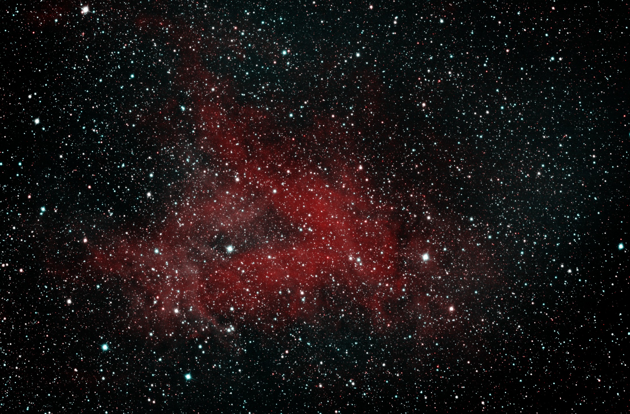
IC1318, commonly known as the Butterfly Nebula, is a vast emission nebula in the constellation Cygnus, spanning over 100 light-years. It is ionized by hot young stars in the Cygnus OB3 association, creating glowing hydrogen clouds and intricate dark dust lanes that give it its distinctive shape. This region exemplifies massive star formation and feedback processes in the galactic plane, with supernova remnants and expanding bubbles sculpting the interstellar medium.
On Earth: ~3,000 BC
The light from IC1318 left around 3000 BC, during the late Neolithic period. In Mesopotamia, the Sumerians were developing early cities like Uruk and inventing cuneiform writing. In Egypt, predynastic cultures were unifying along the Nile, leading to the first pharaohs. Stonehenge's early phases were being constructed in Britain, and agriculture was spreading across Europe and Asia.
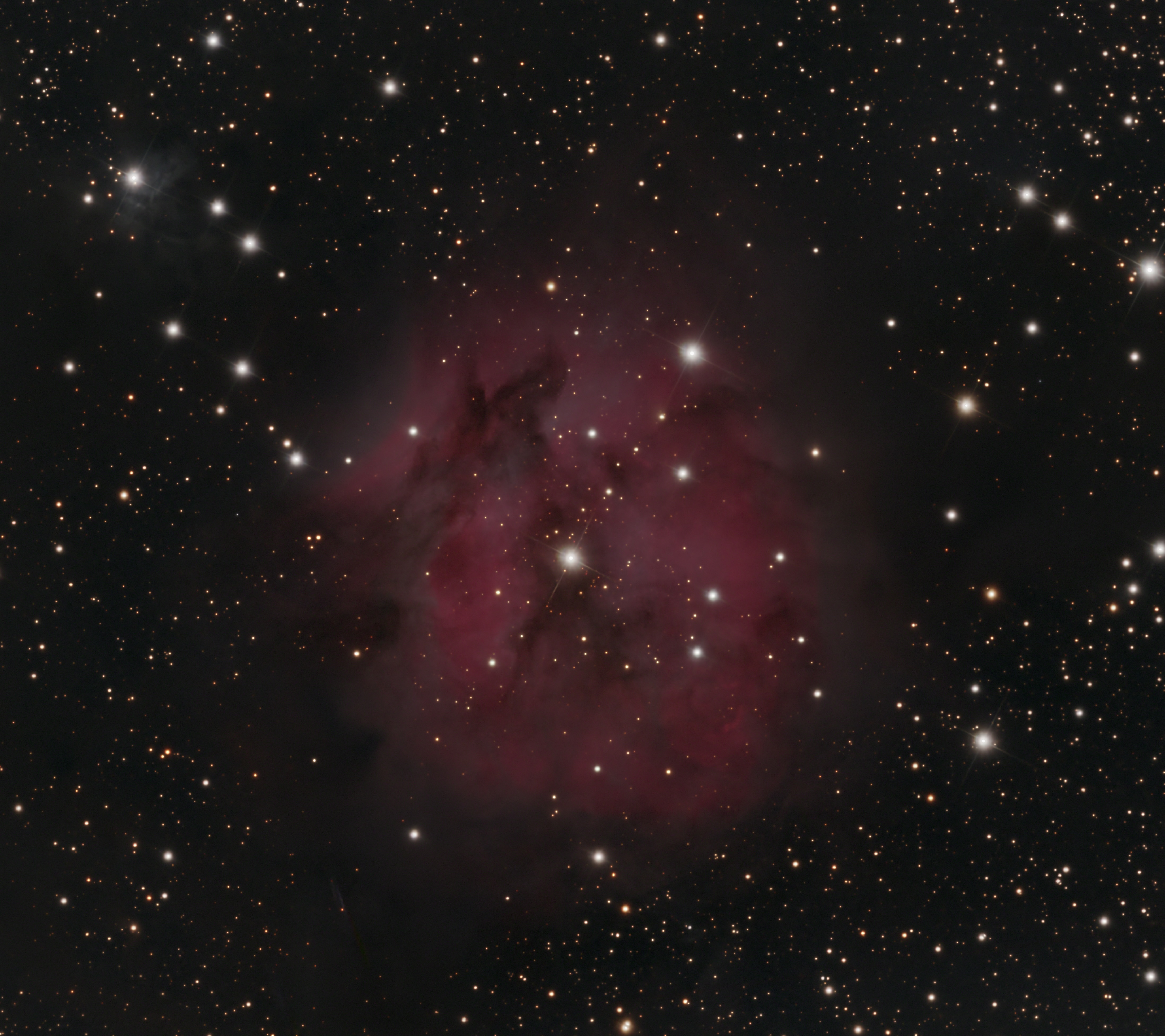
IC5146 - Cocoon Nebula
DISTANCE: ~4,000 LIGHT YEARS | TYPE: EMISSION / REFLECTION NEBULA
IC5146, the Cocoon Nebula, is a young star-forming region in the constellation Cygnus consisting of both an emission nebula and a reflection nebula wrapped around a nascent star cluster. Ionizing radiation from the central hot star BD+46°3474 illuminates and sculpts the surrounding hydrogen gas, producing the nebula's vivid reddish glow, while residual dust reflects bluer starlight. Extending from the Cocoon is a striking dark molecular cloud known as Barnard 168—a dense filament of cold gas and dust that blocks background starlight and represents the raw material from which the cluster recently formed. The system offers a rare glimpse into the transition from a cold dark cloud to an active H II region, capturing stellar birth in near real time on cosmic scales.
On Earth: ~2,000 BC
These photons began their journey during the Early Bronze Age. In Egypt, the Middle Kingdom was flourishing—pharaohs commissioned monumental temples and expanded trade networks deep into Nubia and the Levant. In Mesopotamia, the Third Dynasty of Ur gave way to the rise of Babylon. Meanwhile, the first Indo-European migrations were reshaping the populations of Europe and South Asia, and Stonehenge was receiving its final massive sarsen stones.
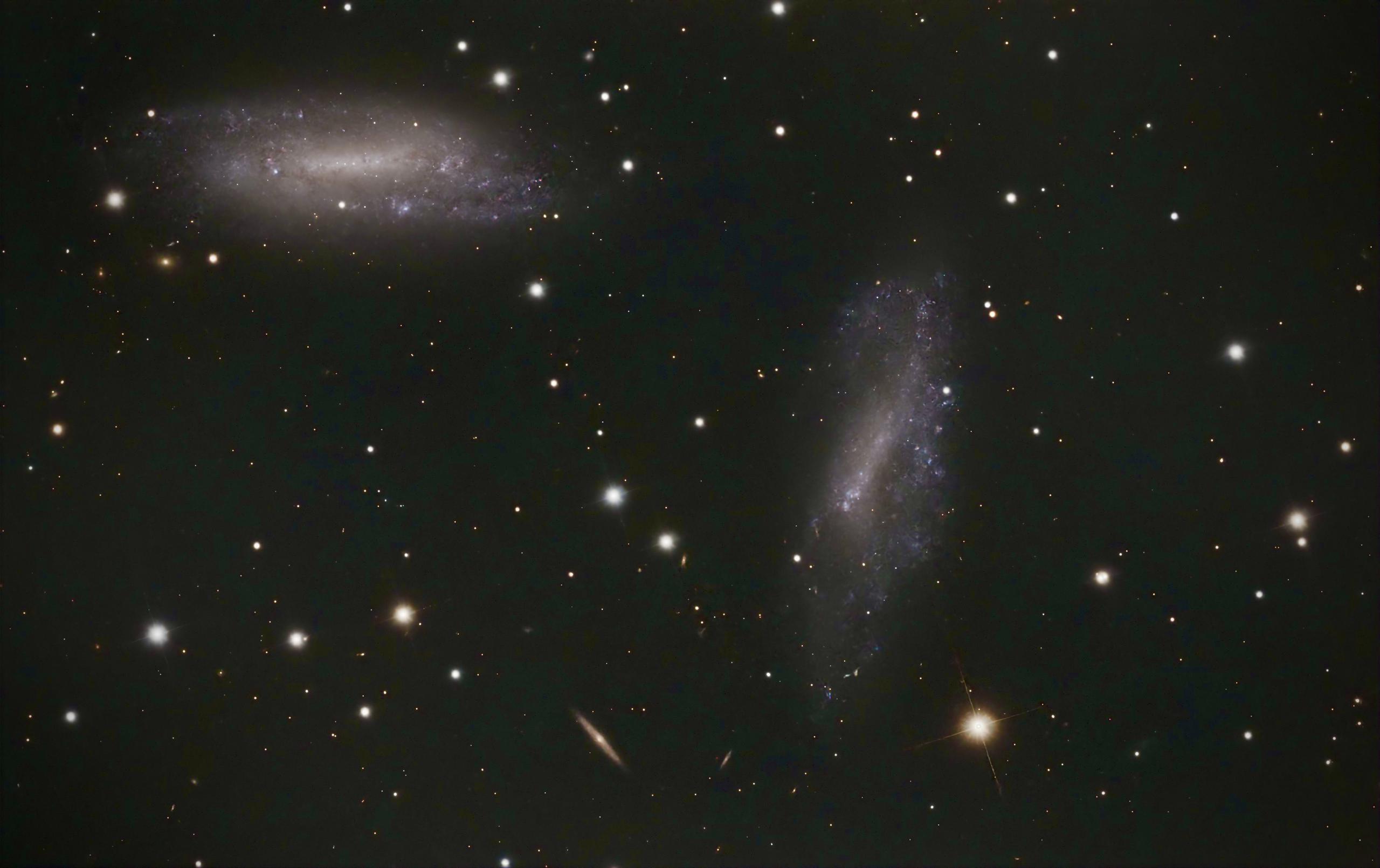
IC727 - Spiral Galaxy
DISTANCE: ~30 MILLION LIGHT YEARS | TYPE: SPIRAL GALAXY
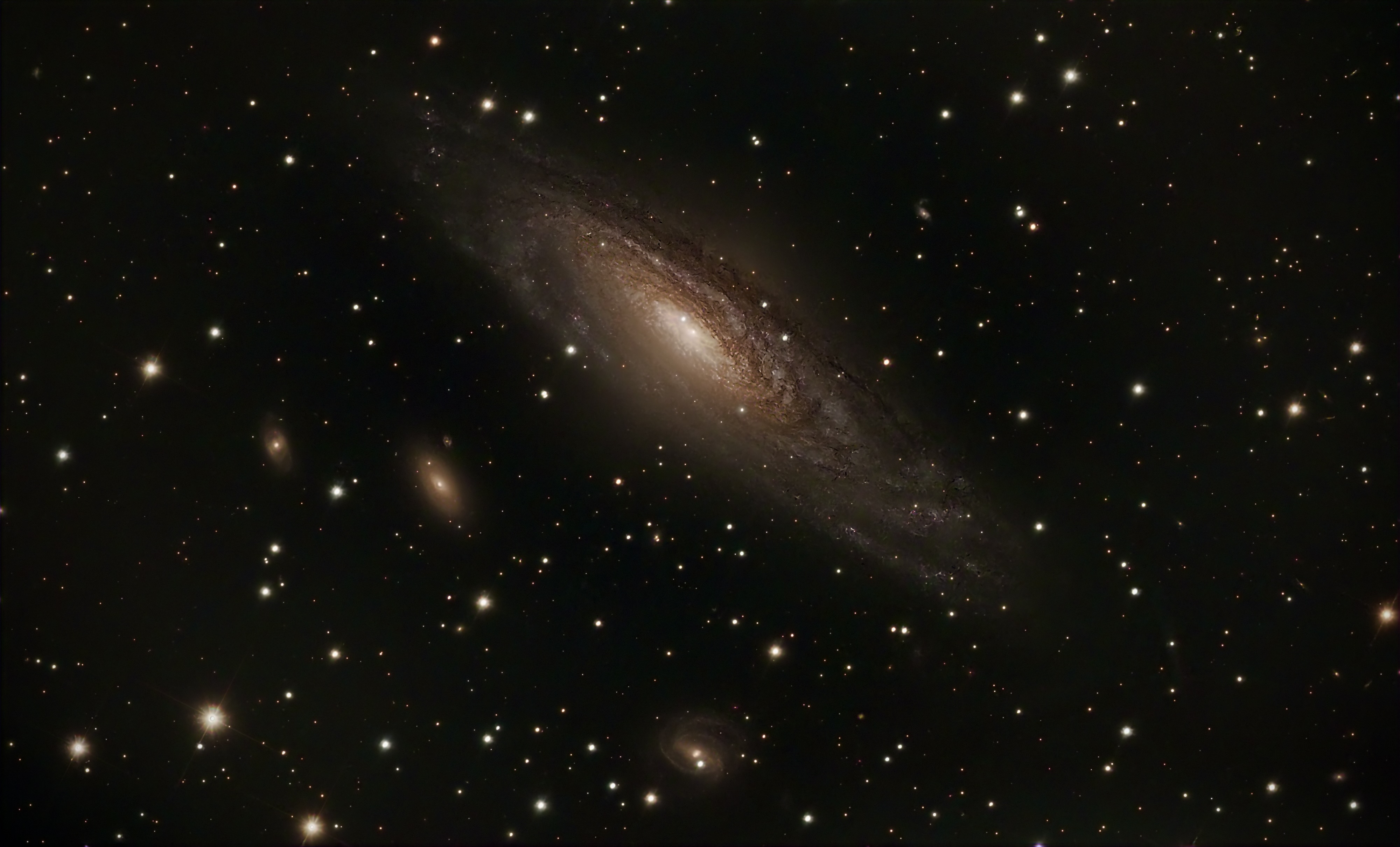
IC727 is a spiral galaxy in the constellation Draco, characterized by its well-defined arms and active star-forming regions. At approximately 30 million light-years, it provides opportunities to study galactic structure and evolution in relative proximity, including supernova remnants and interstellar medium dynamics.
On Earth: 30 Million Years Ago
In the Oligocene epoch, primates diversified with the emergence of early monkeys. The climate cooled, leading to the expansion of grasslands and the evolution of grazing mammals. India continued colliding with Asia, raising the Himalayas, while Antarctica's ice cap began forming.
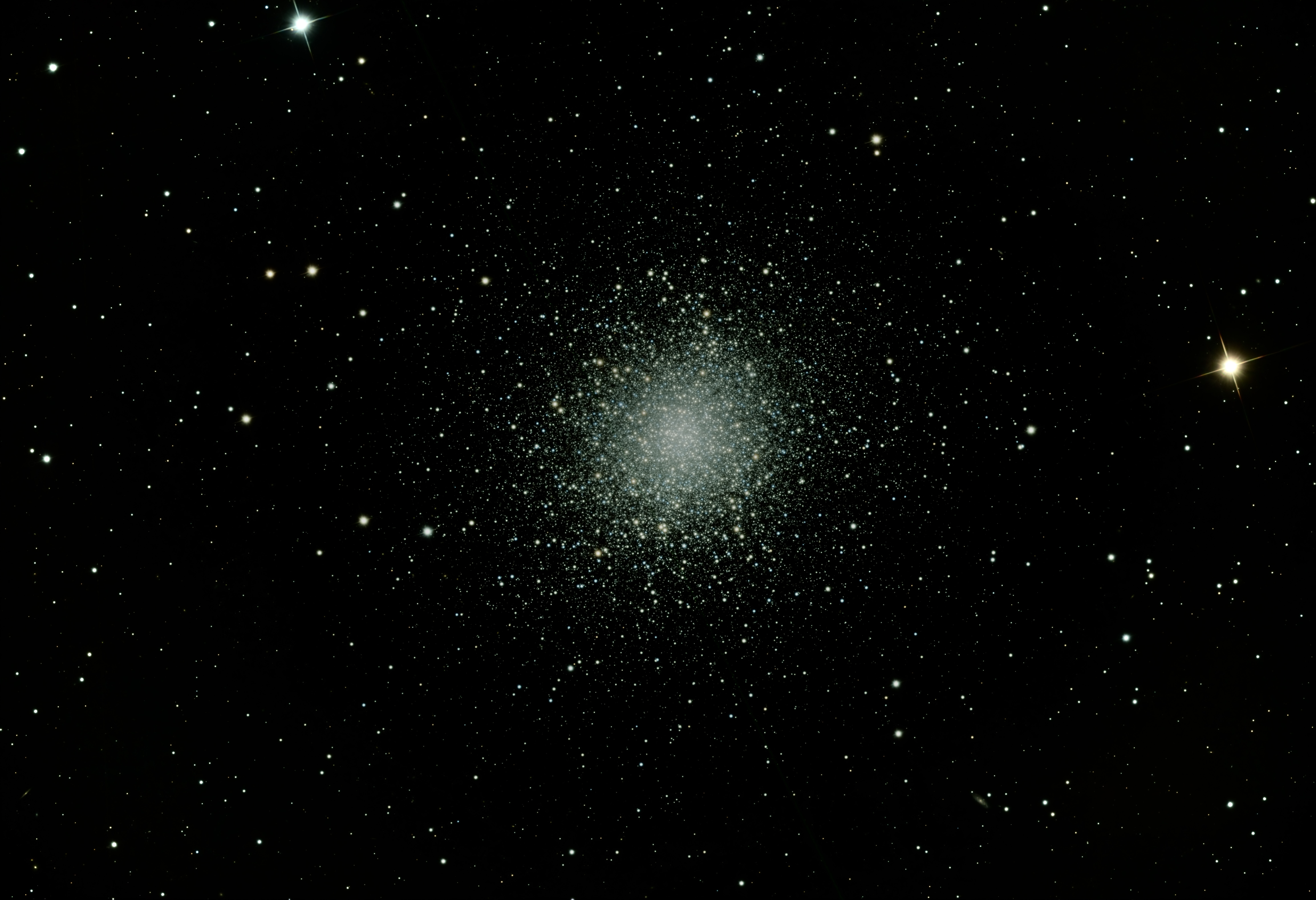
M13 - Hercules Globular Cluster
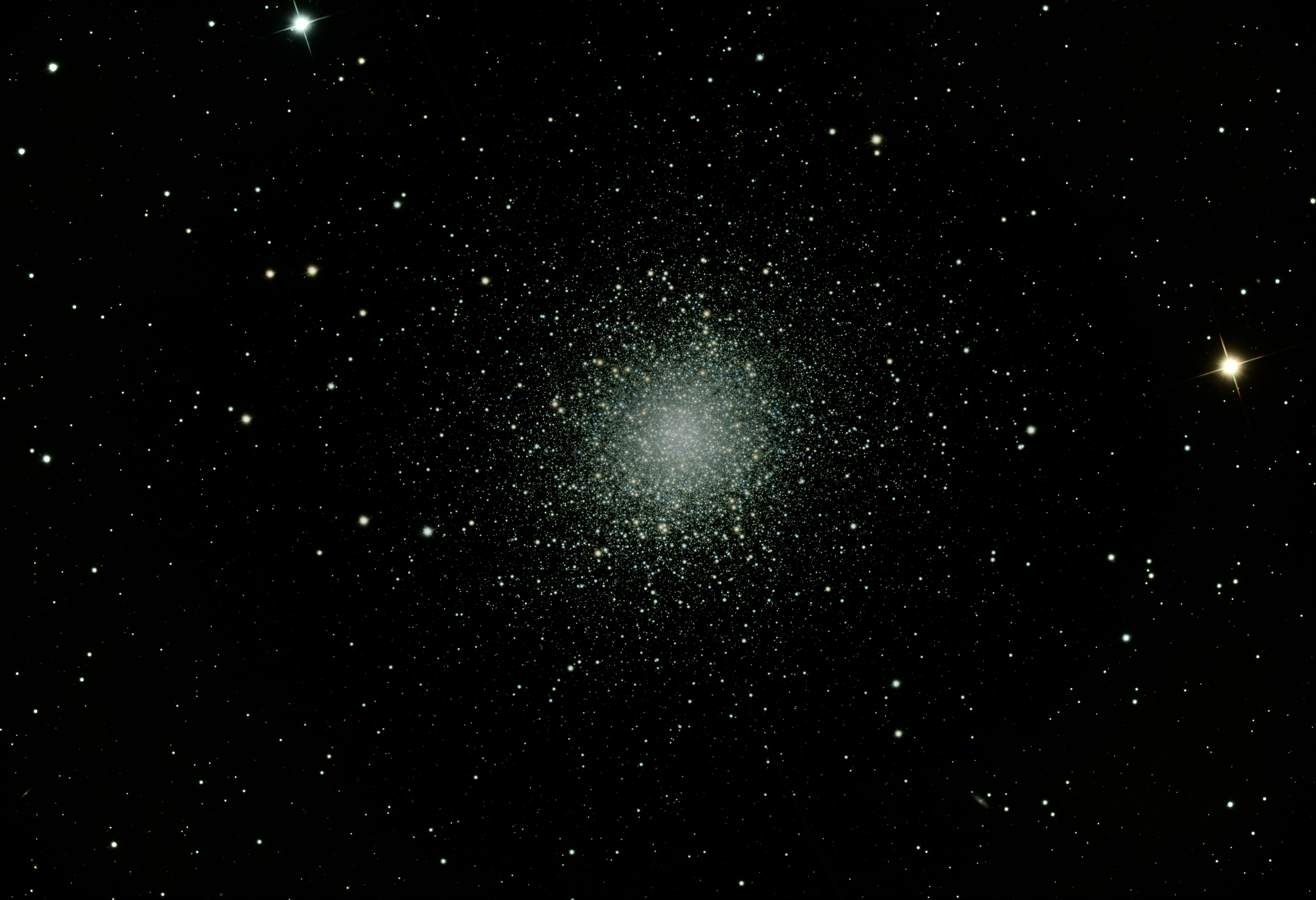
DISTANCE: ~25,000 LIGHT YEARS | TYPE: GLOBULAR CLUSTER
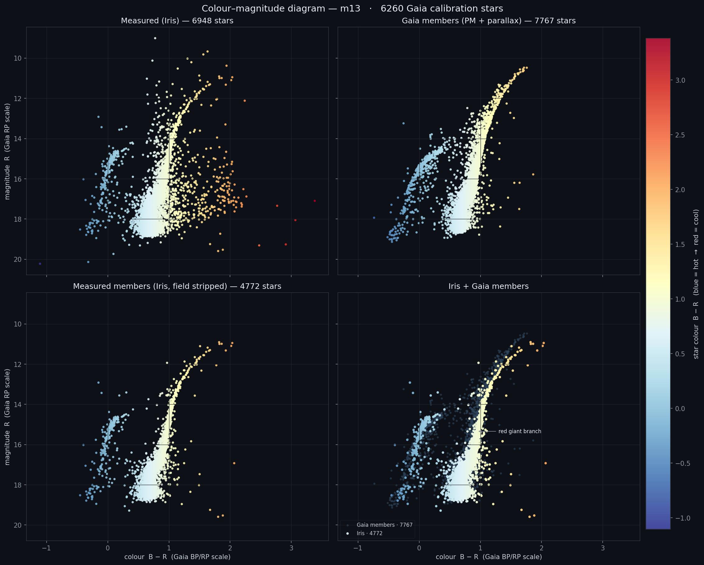
M13 is one of the oldest known globular clusters in the Milky Way, containing over 300,000 stars packed into a 145 light-year diameter sphere. Aged at 11.65 billion years, it orbits the galactic center in a halo trajectory, providing insights into stellar evolution, variable stars, and the galaxy's formation history through its low-metallicity Population II stars.
On Earth: ~23,000 BC
When this light departed M13, Earth was in the Last Glacial Maximum. Modern humans were creating cave art in Europe, like at Lascaux. Hunter-gatherers adapted to ice age conditions, with megafauna like mammoths dominating. The Bering land bridge allowed migration to the Americas.
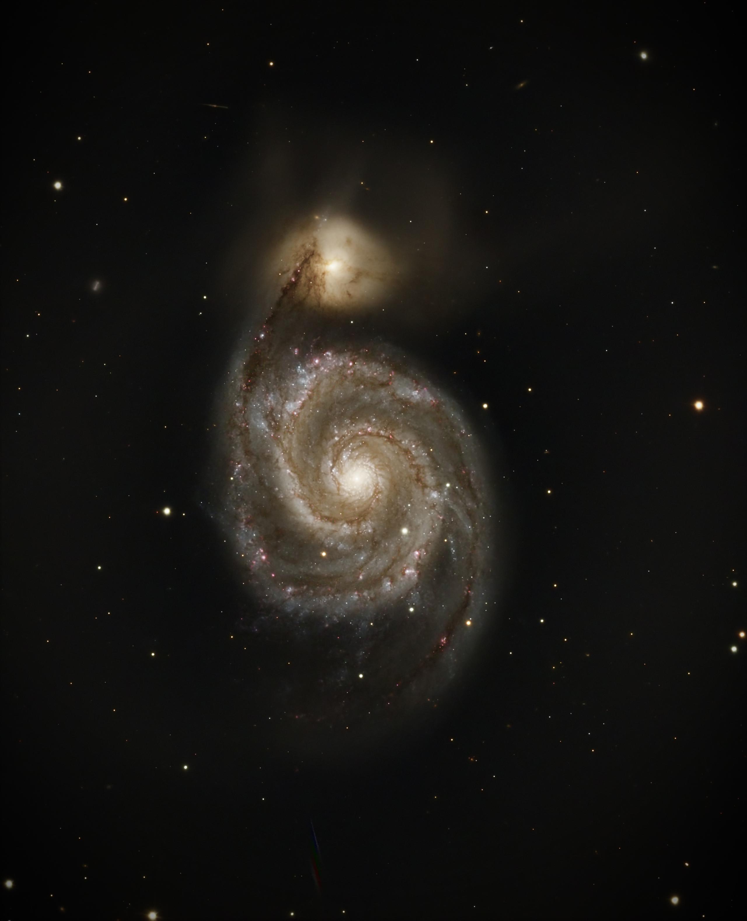
M51 - Whirlpool Galaxy
DISTANCE: ~23 MILLION LIGHT YEARS | TYPE: INTERACTING SPIRAL GALAXY
M51 is a grand-design spiral interacting with companion NGC 5195, triggering enhanced star formation visible in its arms. This system exemplifies tidal interactions, density waves, and galaxy mergers, with a Seyfert nucleus indicating black hole activity.
On Earth: 23 Million Years Ago
The Miocene epoch saw grasslands expand, with early apes diversifying in Africa. Massive sharks like Megalodon ruled the oceans, and the Himalayas rose higher. Continental drift shaped modern geography, with cooling climates setting the stage for future ice ages.
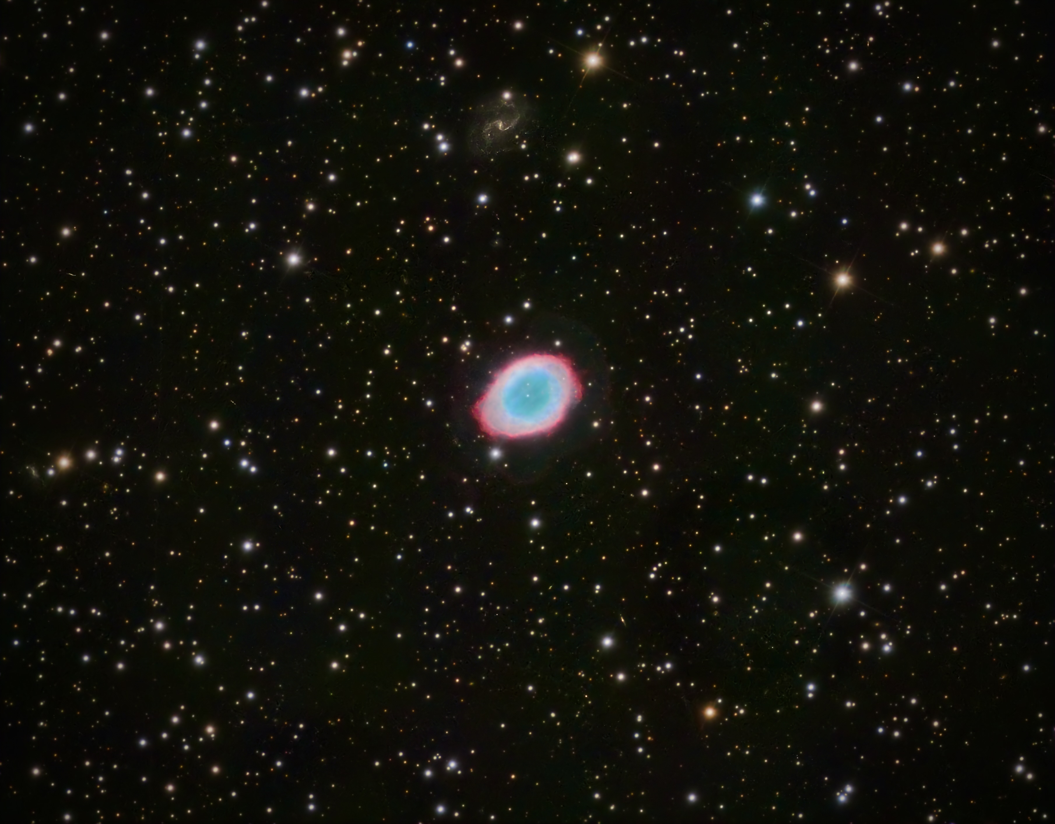
M57 - Ring Nebula
DISTANCE: ~2,300 LIGHT YEARS | TYPE: PLANETARY NEBULA
M57, the Ring Nebula in the constellation Lyra, is one of the sky's most iconic planetary nebulae—a glowing shell of ionized gas expelled by a Sun-like star as it exhausted its nuclear fuel and shed its outer layers. The faint white dwarf at the center, once the star's core, radiates intense ultraviolet light that causes the surrounding gas to fluoresce in concentric rings of oxygen, hydrogen, and nitrogen. While it appears as a simple torus from our vantage point, three-dimensional models reveal a more complex barrel-shaped structure, viewed nearly end-on. M57 represents the inevitable fate of stars like our own Sun, offering a preview—roughly five billion years in the future—of what will become of our solar neighborhood.
On Earth: ~300 BC
These photons departed during the early Hellenistic period, shortly after the death of Alexander the Great. His conquests had spread Greek culture from Egypt to the borders of India, and successor kingdoms—the Ptolemaic, Seleucid, and Antigonid dynasties—were carving up his empire. In China, the Warring States period was drawing to a close as the Qin state steadily consolidated power, just decades away from unifying China under its first emperor. In the Mediterranean, the Roman Republic was expanding southward, laying the groundwork for an empire.
M63 - Sunflower Galaxy
DISTANCE: ~29 MILLION LIGHT YEARS | TYPE: SPIRAL GALAXY
M63 features flocculent spiral arms with patchy star formation. Its active nucleus and ultraviolet excess suggest recent starburst activity, providing insights into spiral structure maintenance without strong density waves.
On Earth: 29 Million Years Ago
The late Oligocene saw the diversification of early elephants and the spread of grasslands. In Antarctica, ice sheets expanded, cooling the planet. Primate evolution accelerated, with ancestors of Old World monkeys appearing.
M74 - Phantom Galaxy
DISTANCE: ~32 MILLION LIGHT YEARS | TYPE: SPIRAL GALAXY
M74 is a face-on grand-design spiral with well-defined arms rich in H II regions. Its low surface brightness and symmetric structure make it a prime target for studying spiral density waves and star formation triggers.
On Earth: 32 Million Years Ago
The Eocene-Oligocene transition brought rapid cooling and mass extinctions of marine life. Early elephants and odd-toed ungulates evolved, while the first Antarctic ice sheets formed, lowering sea levels worldwide.
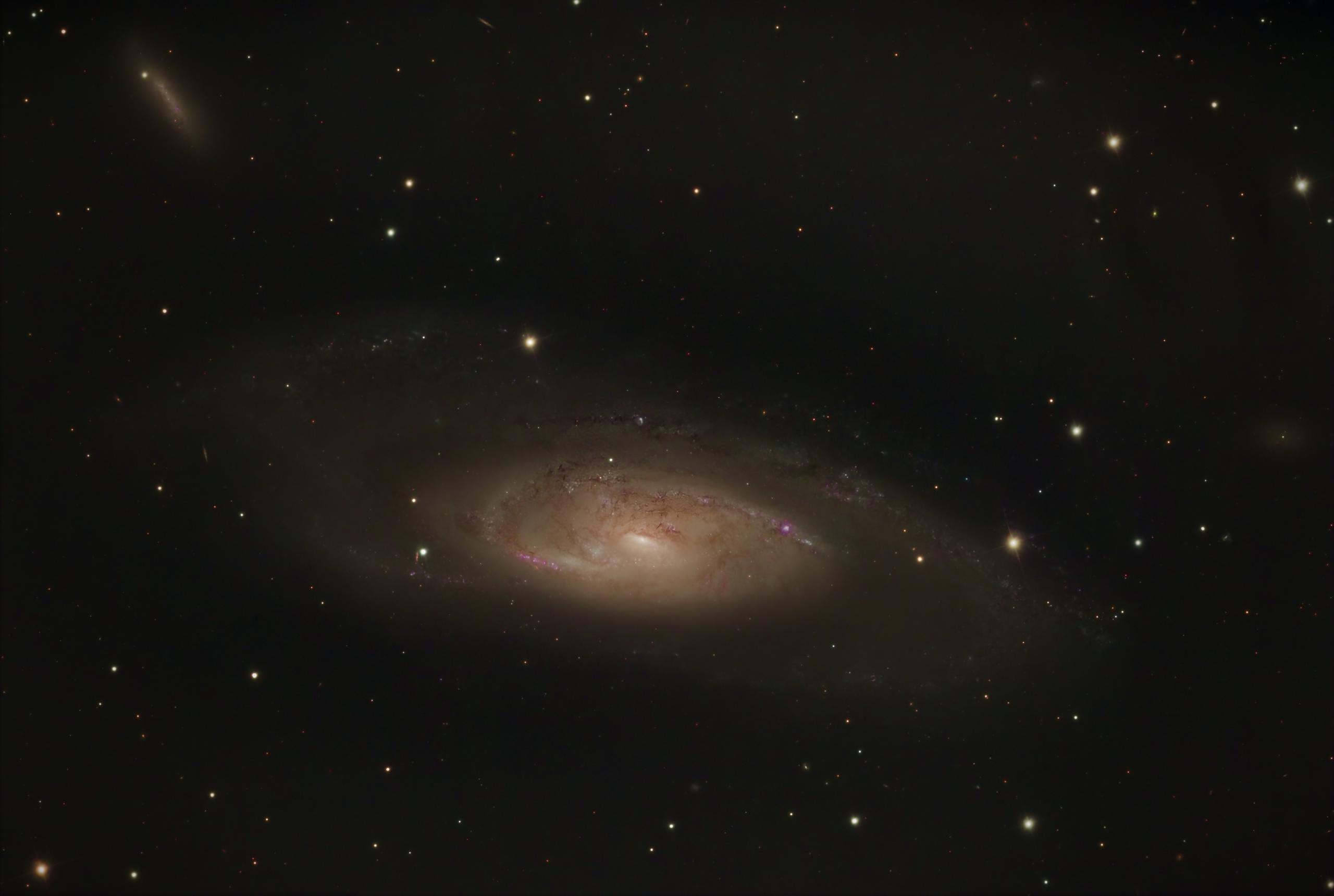
M94 - Croc's Eye Galaxy
DISTANCE: ~16 MILLION LIGHT YEARS | TYPE: SPIRAL GALAXY
M94, nicknamed the Croc's Eye Galaxy, is a compact spiral galaxy in Canes Venatici notable for its unusually bright, starburst-active nucleus ringed by a tightly wound inner disk. Surrounding this inner structure is a broader, faint outer ring of older stellar populations—giving the galaxy a nested, multi-ring architecture rarely so clearly displayed. The intense star formation in the inner ring is thought to be driven by a density wave resonance rather than a galaxy merger, making M94 a valuable case study in internally triggered starbursts. Its relatively face-on orientation allows astronomers to map the transition zones between these distinct stellar populations in fine detail.
On Earth: 16 Million Years Ago
These photons left during the middle Miocene, an era of exceptional warmth known as the Miocene Climatic Optimum. Vast subtropical forests stretched across Europe and North America, supporting diverse faunas of early apes, three-toed horses, and mastodons. In East Africa, the ancestors of humans were beginning to diverge from other great ape lineages. The Himalayan and Alpine mountain-building was in full swing, gradually reshaping ocean circulation and setting the stage for the planet's long cooling trend toward the Ice Ages.
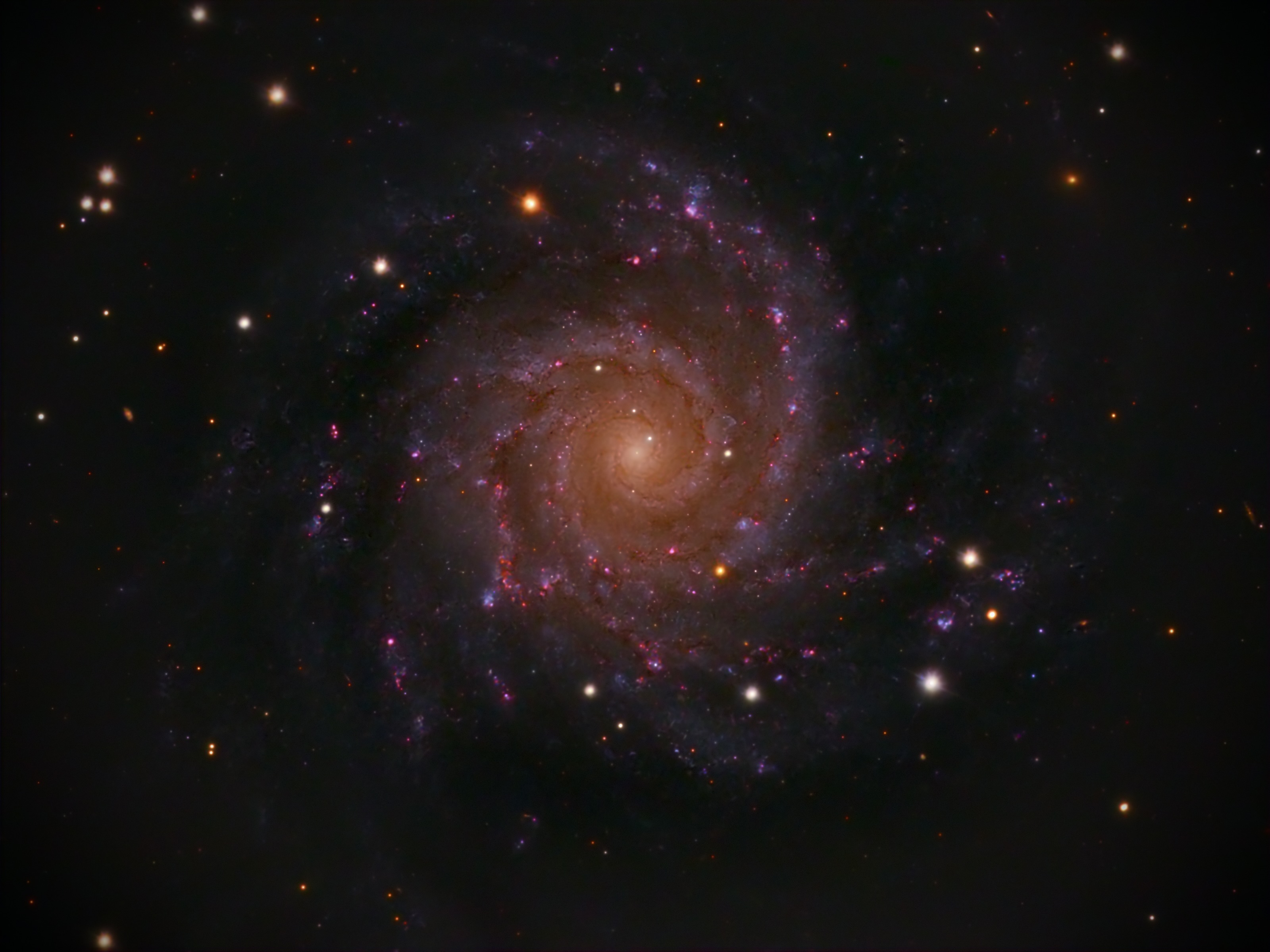
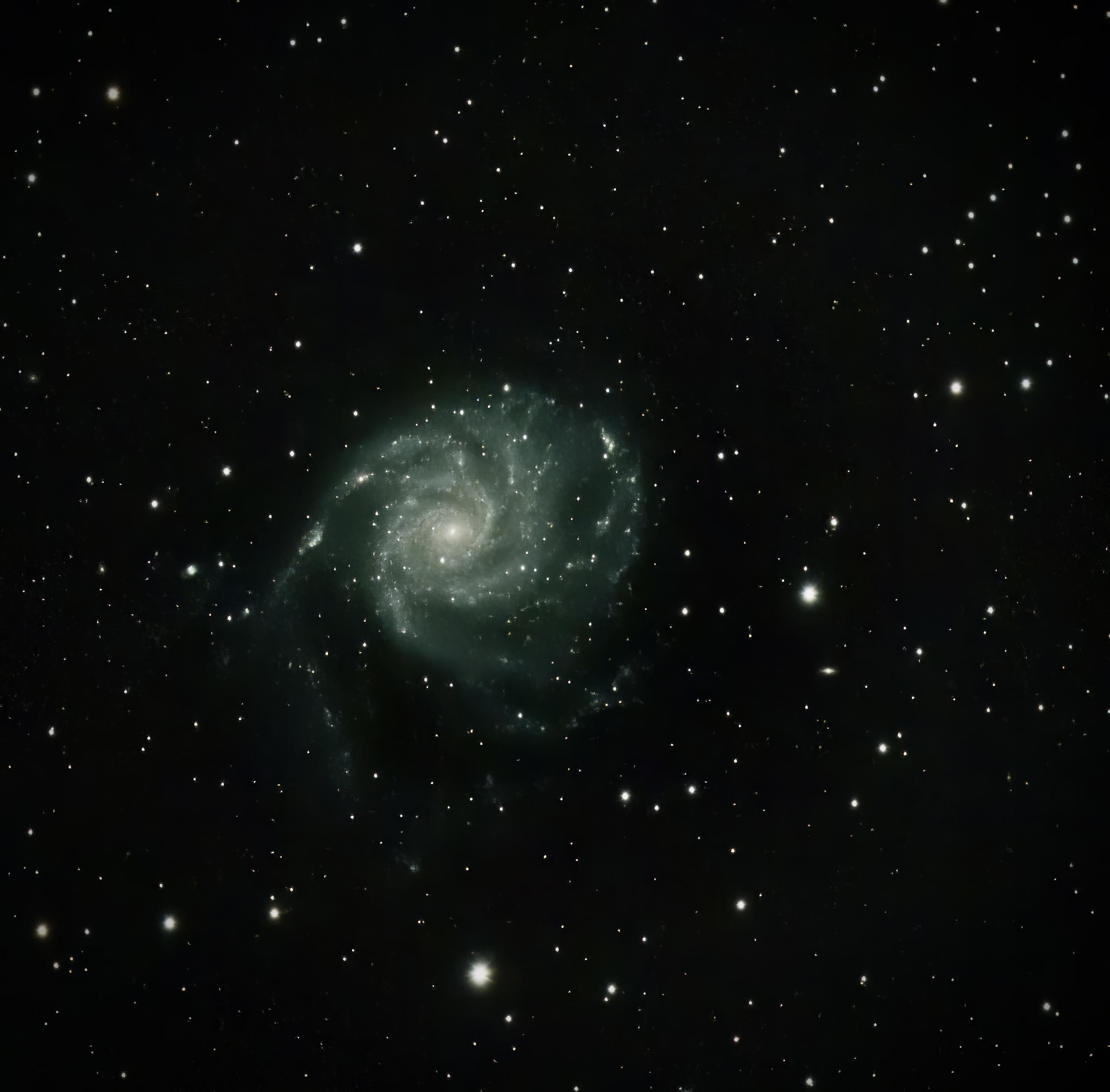
M101 - Pinwheel Galaxy
DISTANCE: ~21 MILLION LIGHT YEARS | TYPE: SPIRAL GALAXY
M101 is a grand-design spiral with asymmetric arms possibly due to interactions with companions. Hosting numerous H II regions, it has a high supernova rate, making it ideal for studying star formation and galactic asymmetry.
On Earth: 21 Million Years Ago
In the Miocene, apes proliferated in Africa and Eurasia. Grasslands expanded, leading to the evolution of modern horses and elephants. The Mediterranean Sea experienced desiccation events, and global temperatures began a long-term cooling trend.
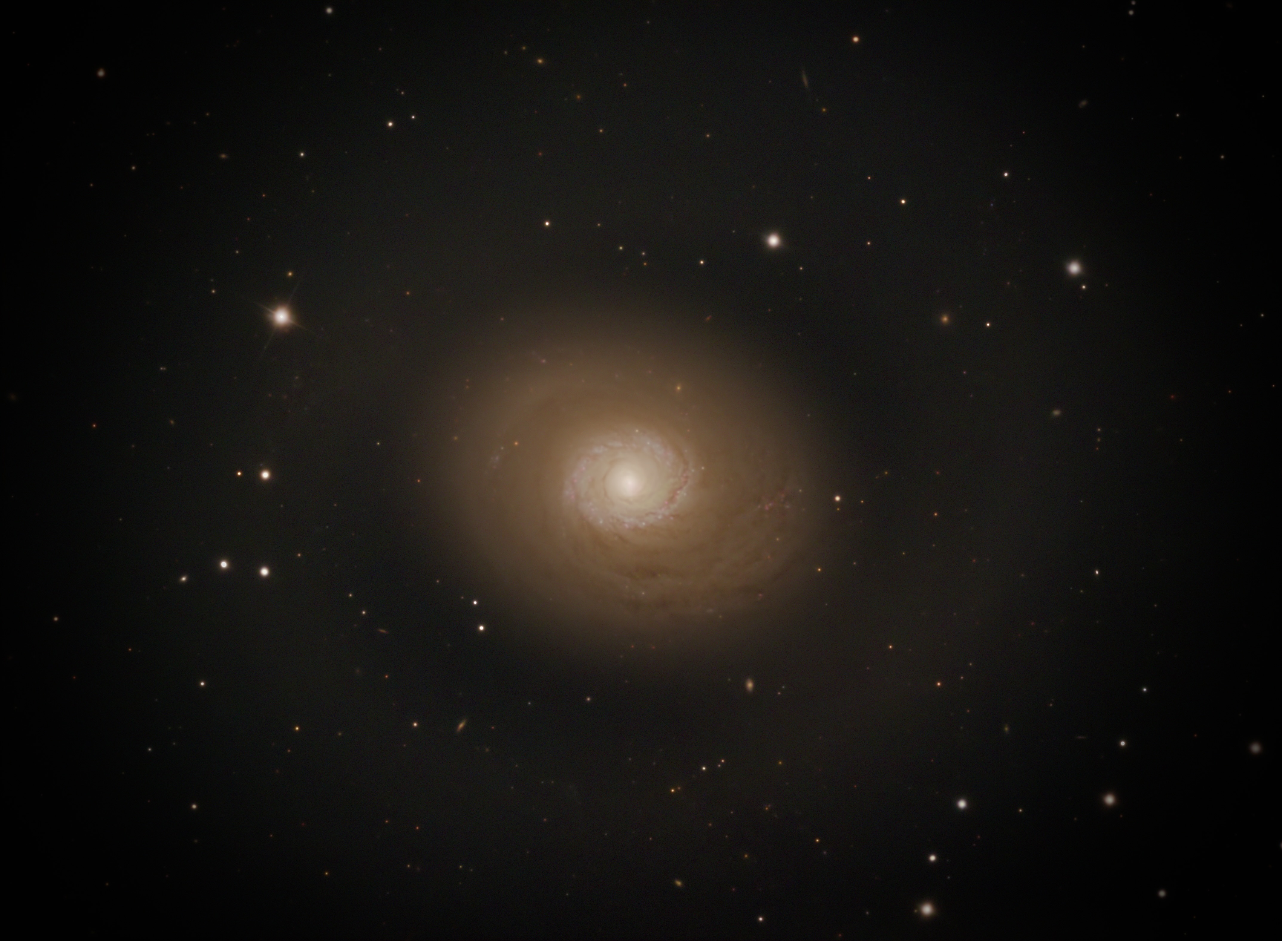
M106 - Spiral Galaxy
DISTANCE: ~23.5 MILLION LIGHT YEARS | TYPE: SPIRAL GALAXY
M106 is a Seyfert spiral with anomalous arms of hot gas, likely ejected from its active nucleus. This LINER galaxy demonstrates feedback from supermassive black holes, influencing star formation and galactic evolution.
On Earth: 23.5 Million Years Ago
Early Miocene saw the diversification of grazing animals as grasslands spread. Apes migrated from Africa to Eurasia, and massive volcanic eruptions formed the Columbia River Basalts. Global cooling continued, leading to Antarctic glaciation.
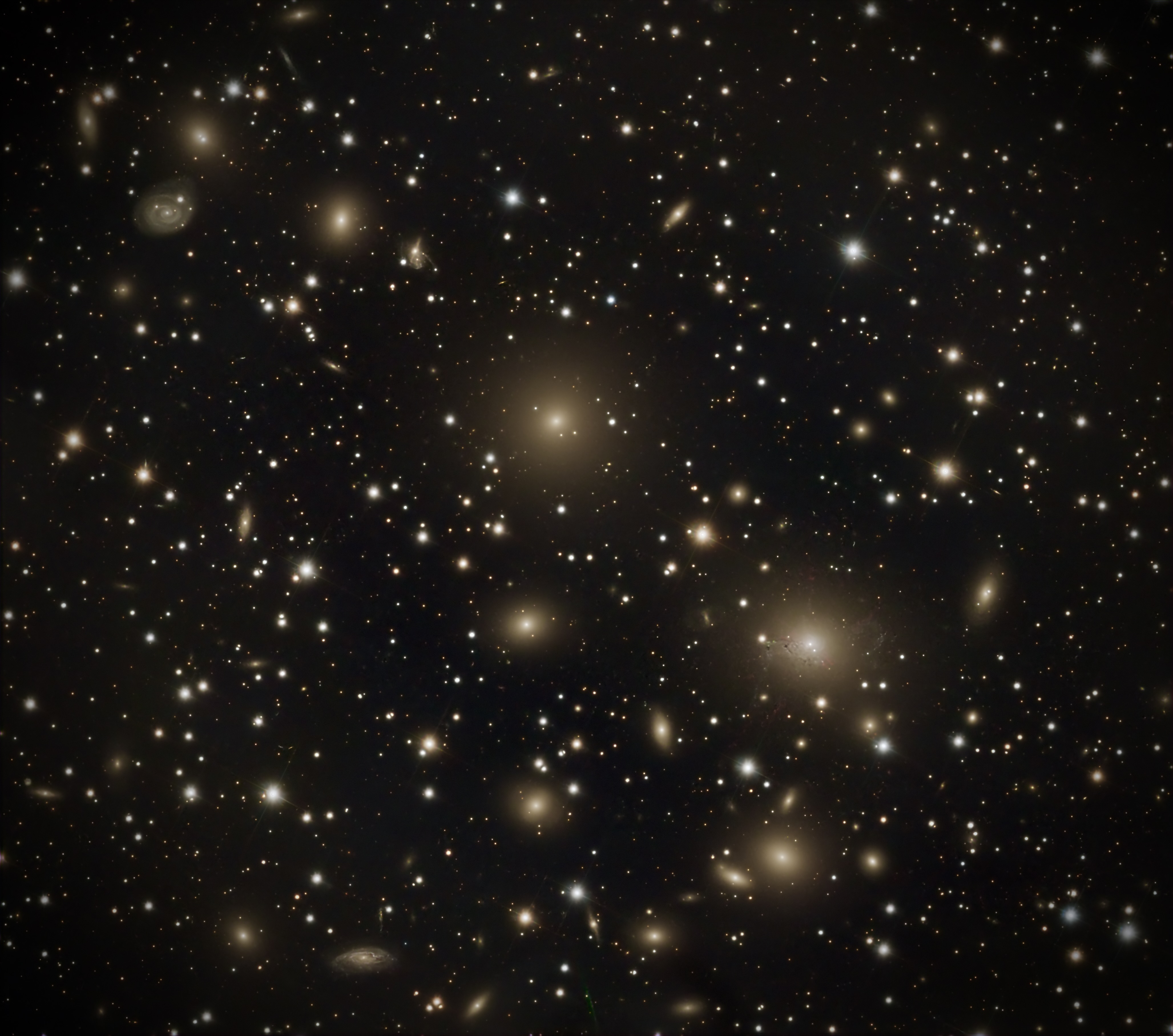
NGC1275 - Perseus A
DISTANCE: ~230 MILLION LIGHT YEARS | TYPE: SEYFERT GALAXY
NGC1275 is the dominant galaxy in the Perseus Cluster, a radio galaxy with an active nucleus powered by a supermassive black hole. It exhibits filamentary structures of cool gas falling into the hot intracluster medium, providing key evidence for AGN feedback mechanisms that regulate star formation and cluster cooling flows.
On Earth: 230 Million Years Ago
The photons left during the Triassic period, when the supercontinent Pangaea was forming. Early dinosaurs and mammals were emerging after the Permian extinction. Vast forests of cycads and ferns covered the land, and the first flying reptiles appeared in a world recovering from mass extinction.
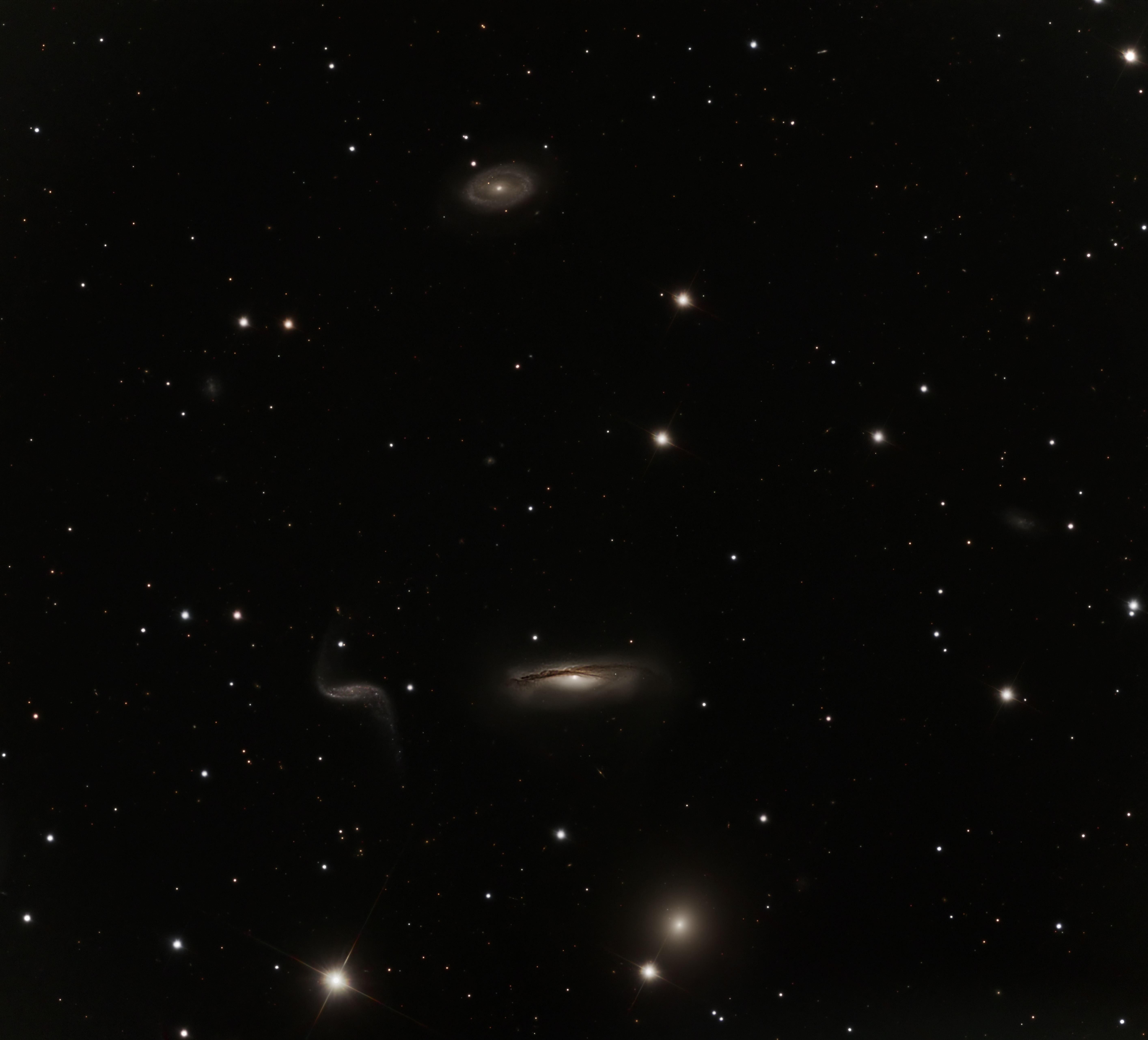
NGC3190 - Hickson Compact Group 44
DISTANCE: ~70 MILLION LIGHT YEARS | TYPE: INTERACTING SPIRAL GALAXY GROUP
NGC3190 is the most prominent member of Hickson Compact Group 44 (HCG 44) in Leo—a tight knot of four gravitationally bound galaxies whose mutual interactions are visibly warping their structures. NGC3190 itself is an edge-on spiral with a striking, sharply twisted dust lane, the result of tidal forces from its neighbors. Compact groups like HCG 44 are among the densest galaxy environments known, where repeated close encounters strip gas, trigger starbursts, and ultimately drive galaxies toward merger. The group serves as a local laboratory for understanding how environment accelerates galactic evolution, a process that shaped much of the large-scale structure of the universe.
On Earth: 70 Million Years Ago
These photons left Earth during the twilight of the age of dinosaurs—roughly five million years before the Chicxulub asteroid impact that ended the Cretaceous. Tyrannosaurus rex and Triceratops were roaming what is now North America, while mosasaurs ruled shallow inland seas. Flowering plants had transformed terrestrial ecosystems over the preceding tens of millions of years, and small insectivorous mammals were quietly diversifying in the undergrowth, poised to inherit the Earth.
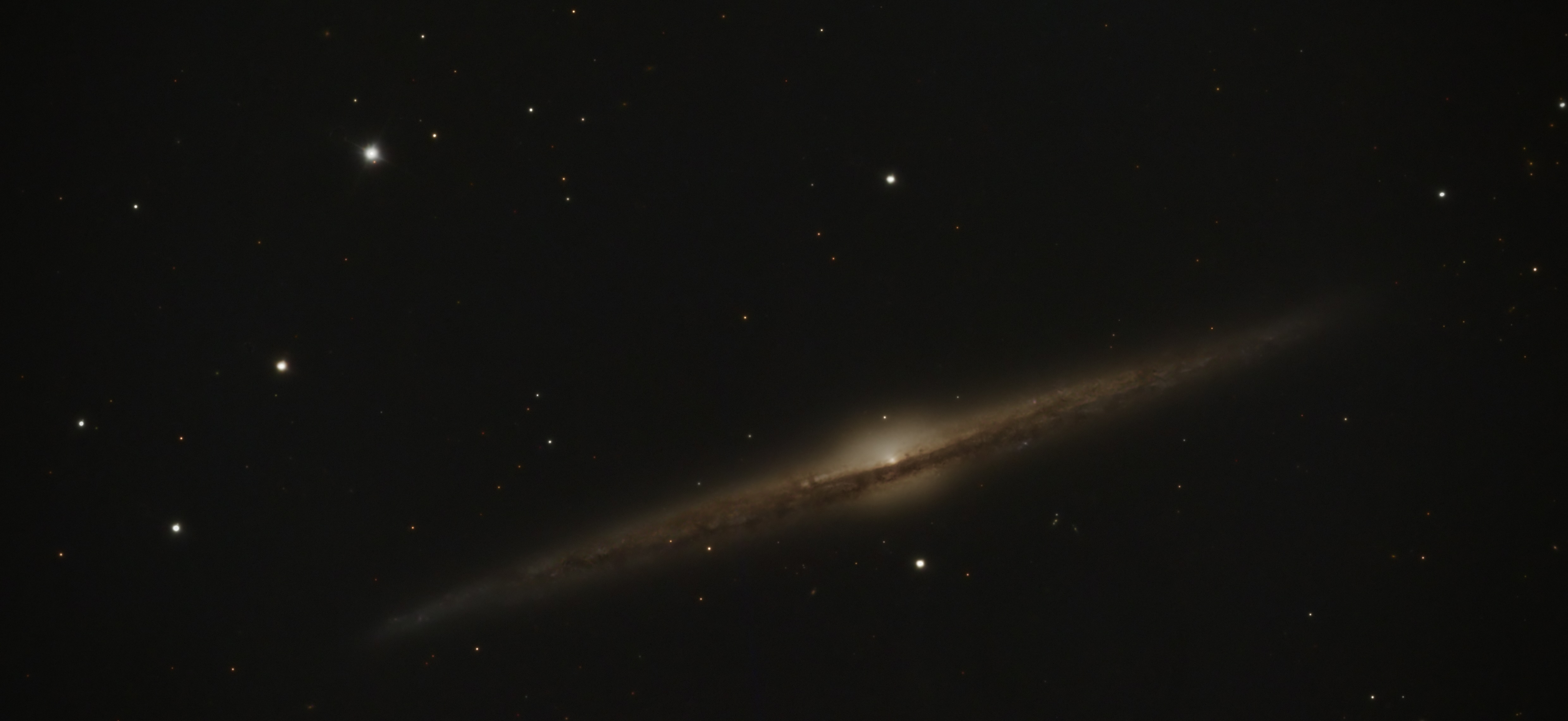
NGC4565 - Needle Galaxy
DISTANCE: ~47 MILLION LIGHT YEARS | TYPE: SPIRAL GALAXY
NGC4565 is an edge-on spiral showcasing a prominent dust lane bisecting its thin disk. Similar in size to the Milky Way, it allows detailed study of galactic structure, including bulge-to-disk ratios and dark matter halo effects through rotation curve analysis.
On Earth: 47 Million Years Ago
During the Eocene, Earth had a greenhouse climate with palm trees in polar regions. Early whales evolved from land mammals, and primates began diversifying. Massive volcanic activity in the North Atlantic formed new ocean basins.
NGC6339 - Spiral Galaxy
DISTANCE: ~94 MILLION LIGHT YEARS | TYPE: SPIRAL GALAXY
NGC6339 is a barred spiral in Hercules with disturbed arms indicating possible interactions. Its kinematics show perpendicular rotation to its major axis, making it valuable for studying galactic bars and secular evolution.
On Earth: 94 Million Years Ago
During the Late Cretaceous, dinosaurs like Tyrannosaurus roamed while flowering plants diversified. The Western Interior Seaway divided North America, and birds began evolving from theropods. The stage was set for the Chicxulub impact.
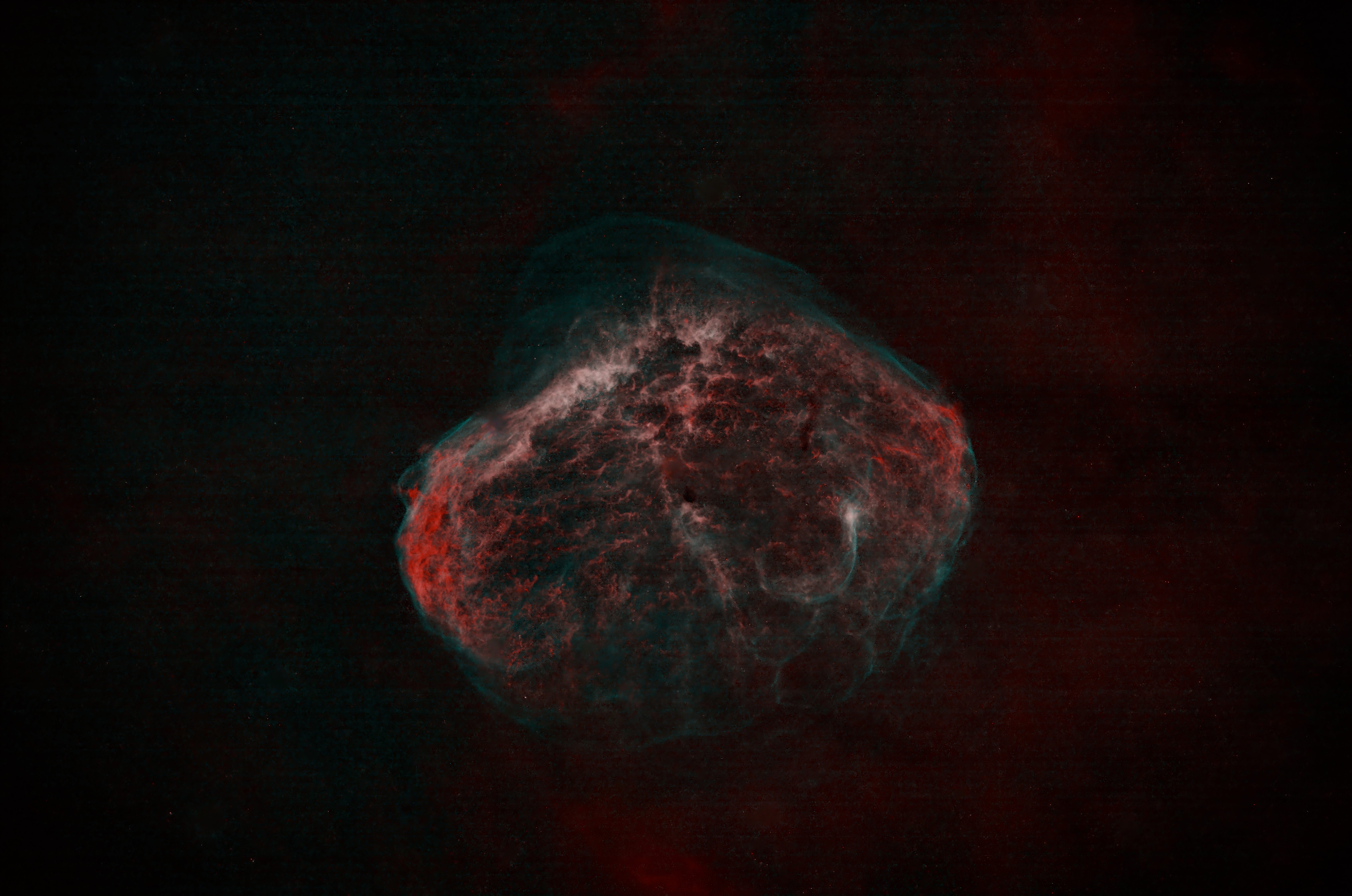
NGC6888 - Crescent Nebula
DISTANCE: ~5,000 LIGHT YEARS | TYPE: EMISSION NEBULA
NGC6888 is a wind-blown bubble formed by the Wolf-Rayet star WR 136, with fast stellar winds colliding with slower red giant ejecta. This 25 light-year shell illustrates late-stage stellar evolution and nebular dynamics.
On Earth: ~3,000 BC
Similar to IC1318's era, this was the time of early Bronze Age civilizations. In Egypt, the Old Kingdom began pyramid construction. Sumerians developed urban centers, and the Indus Valley Civilization emerged with advanced city planning.
NGC7331 - Deer Lick Galaxy
DISTANCE: ~40 MILLION LIGHT YEARS | TYPE: SPIRAL GALAXY
NGC7331 is an unbarred spiral galaxy often compared to the Milky Way, with a prominent dust lane and active star formation in its arms. As the brightest member of its group, it showcases galactic interactions and serves as a calibrator for the cosmic distance ladder through its Cepheid variables.
On Earth: 40 Million Years Ago
During the Eocene epoch, Earth experienced a warm climate with lush forests extending to the poles. Early primates evolved in these environments, while modern mammal orders like whales transitioned from land to sea. Antarctica began separating from Australia, initiating global cooling trends.
NGC7635 - Bubble Nebula
DISTANCE: ~7,100 LIGHT YEARS | TYPE: EMISSION NEBULA
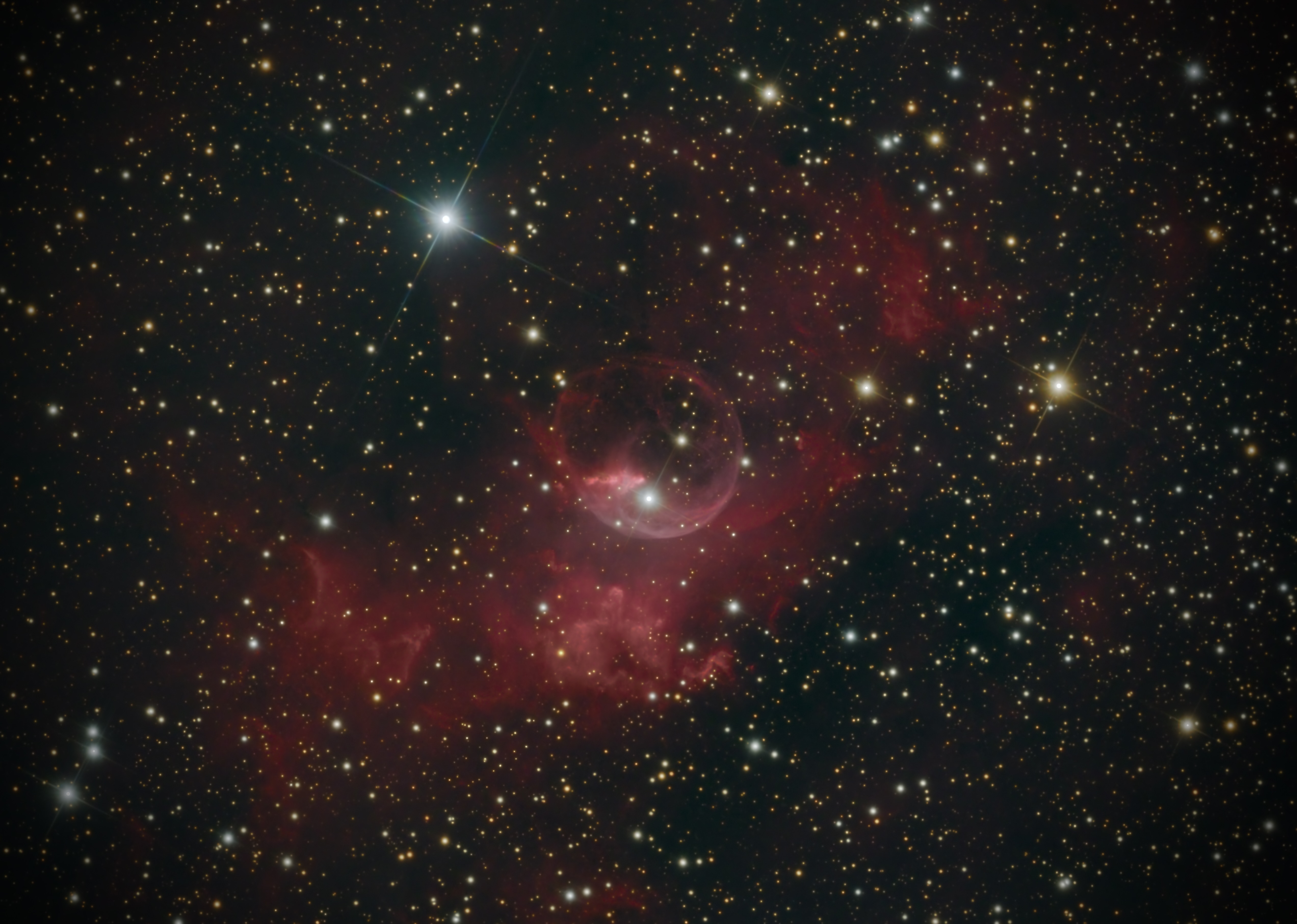
NGC7635 is a spherical shell created by the stellar wind from a massive O-type star, expanding into the surrounding molecular cloud. This 7 light-year diameter bubble demonstrates wind-blown nebula formation and ionization processes in H II regions.
On Earth: ~5,100 BC
The Neolithic period saw the rise of farming villages in the Middle East. Pottery and weaving advanced, and early metallurgy began with copper. In Europe, megalithic tombs were constructed, marking the transition from hunter-gatherer societies.
NGC891 - Silver Sliver Galaxy
DISTANCE: ~30 MILLION LIGHT YEARS | TYPE: SPIRAL GALAXY
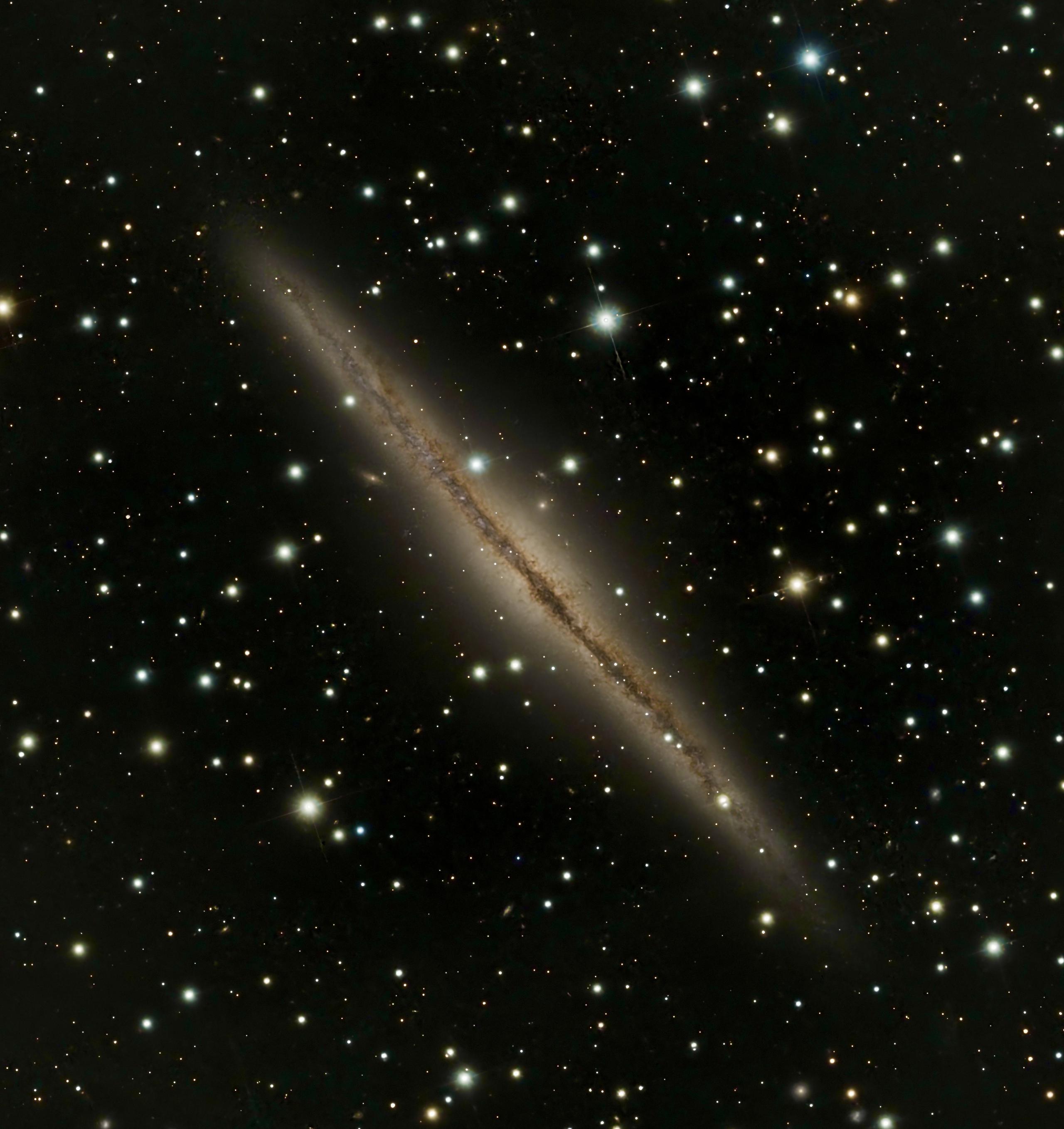
NGC891 is an edge-on spiral with a thick dust lane, similar to how the Milky Way might appear from outside. It reveals vertical structures in its disk, informing models of galactic fountains and the role of magnetic fields in halo gas dynamics.
On Earth: 30 Million Years Ago
The Oligocene featured the rise of modern mammal families. Early whales diversified in the oceans, and the first grasses appeared, transforming ecosystems. Tectonic activity continued shaping continents, with Australia separating from Antarctica.
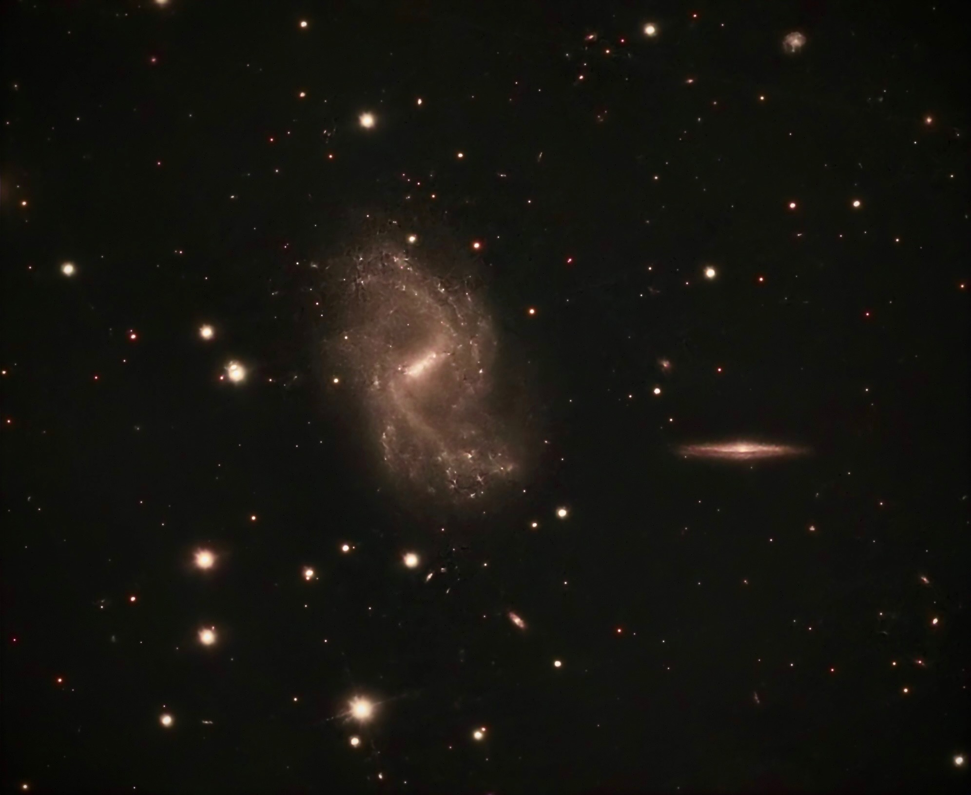
NGC925 - Barred Spiral Galaxy
DISTANCE: ~30 MILLION LIGHT YEARS | TYPE: BARRED SPIRAL GALAXY
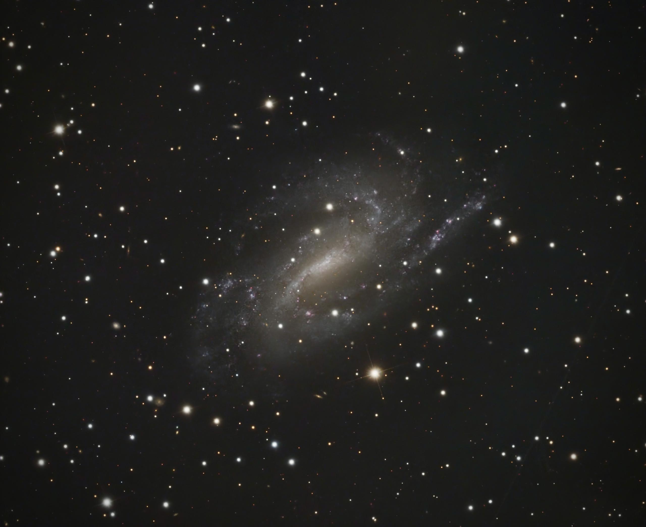
NGC925 is a late-type barred spiral with asymmetric arms and low star formation rate. Part of the NGC 1023 group, it exhibits tidal distortions, useful for studying environmental effects on galaxy morphology and evolution.
On Earth: 30 Million Years Ago
The Oligocene epoch featured the evolution of early cats and dogs. Massive birds like terror birds dominated South America. Global cooling led to the retreat of tropical forests and the rise of temperate ecosystems.
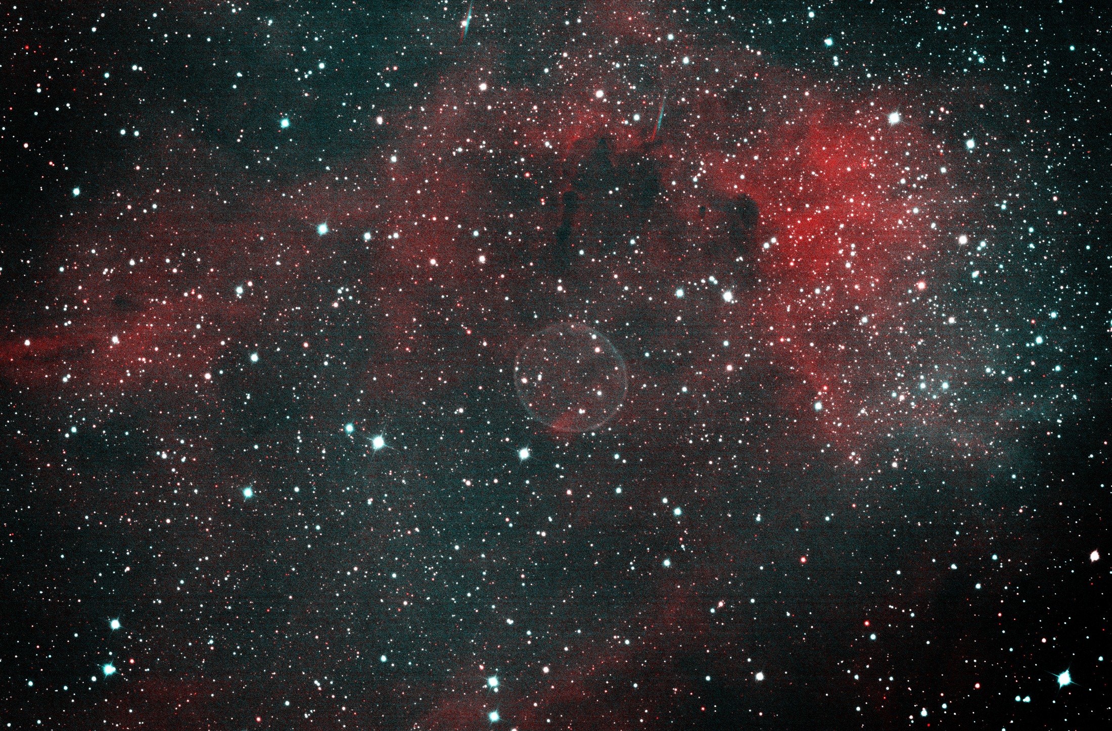
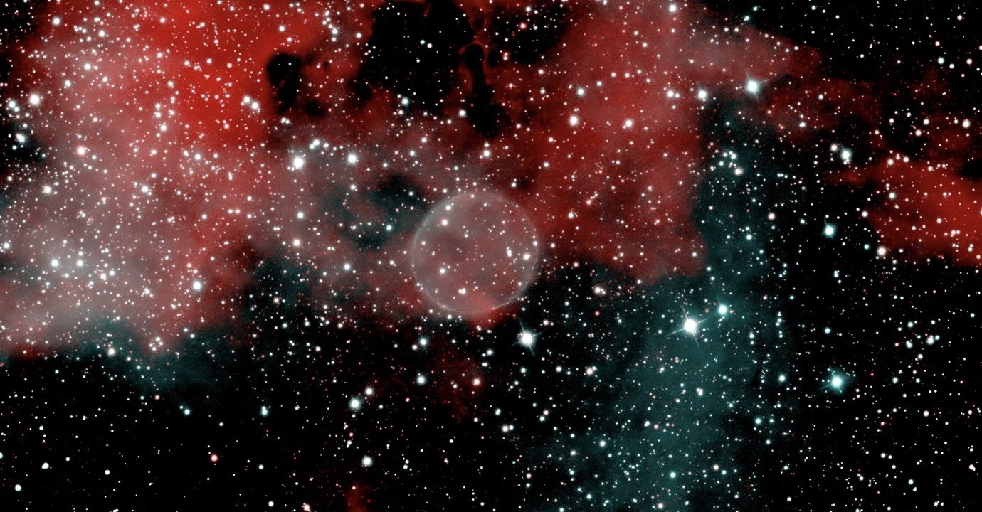
PN G75.5+1.7 - Soap Bubble Nebula
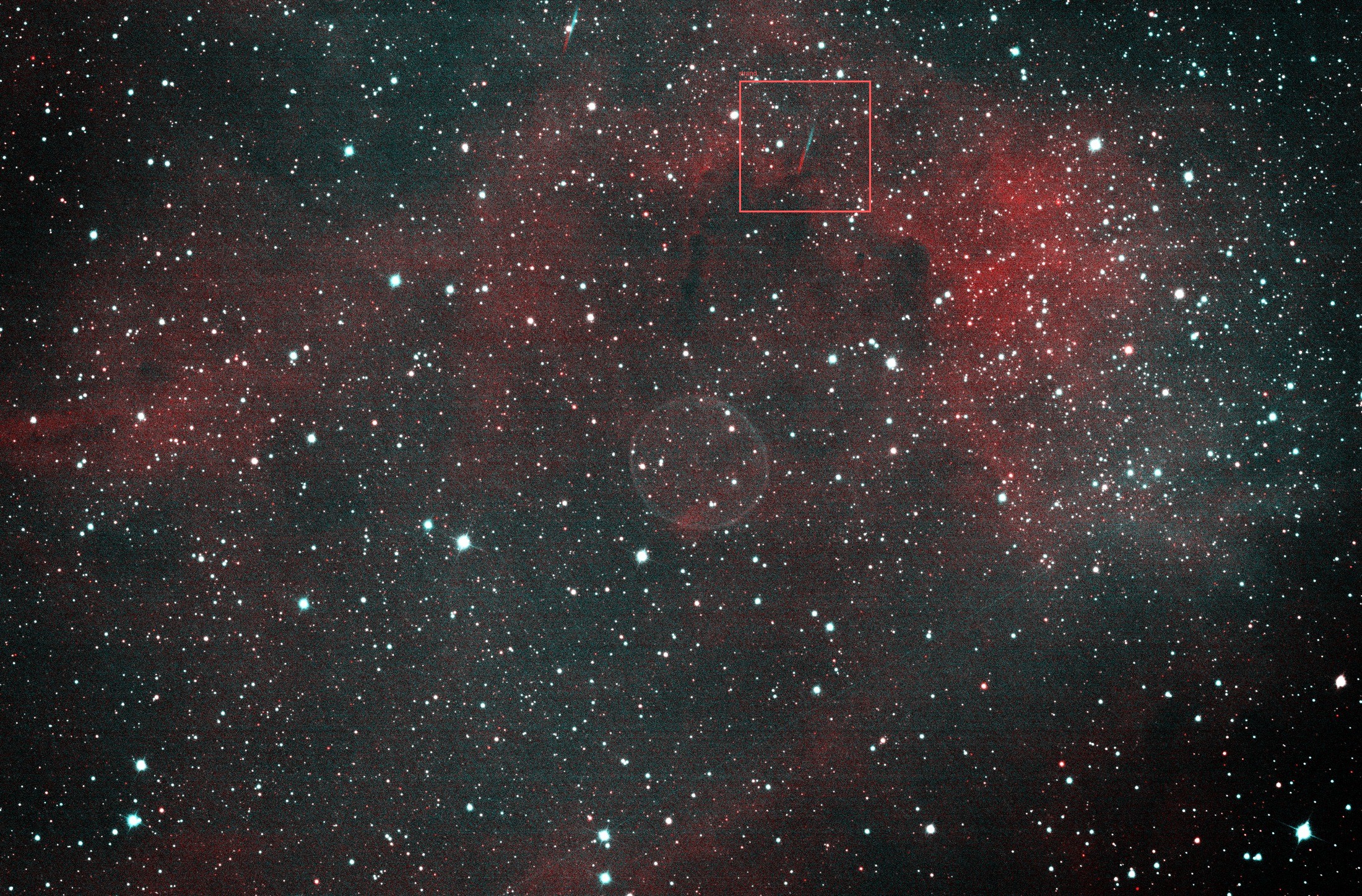
TYPE: PLANETARY NEBULA | 40 Ha + 50 O III × 300 s | 7.5 HOURS | NO HUMAN IN THE LOOP
A planetary nebula in Cygnus, and a genuinely difficult one: it was not
discovered until 2008, because it is a thin spherical shell of very low
surface brightness sitting in front of one of the brightest, most crowded
stretches of the Milky Way. It is the faint teal ring left of centre here.
Everything red around it is unrelated foreground hydrogen in the same line
of sight.
The image is HOO: two narrowband filters instead of red,
green and blue. Hydrogen-alpha at 656.3 nm and doubly ionised oxygen
at 500.7 nm, each passing a band a few nanometres wide. Almost
everything else is rejected before it reaches the sensor — skyglow,
moonlight, the sodium and LED lines of every streetlight for miles. That
is what makes a shell this faint recoverable from a suburban sky at all.
Two filters are then mapped to three channels: hydrogen to red, oxygen to
green and blue together. Nothing feeds green on its own, so pure
green cannot appear; oxygen reads as teal, and the colour of any pixel is
really a ratio between two emission lines.
Those two lines are a map of energy rather than of composition. Freeing an
electron from hydrogen takes 13.6 eV; when one is recaptured it
cascades back down, and the n=3→2 step emits the 656.3 nm photon.
Hydrogen-alpha therefore traces the whole reach of the ultraviolet.
Stripping oxygen twice takes 35.1 eV — nearly three
times as much — and photons that hard are absorbed quickly, so
doubly ionised oxygen survives only near a hot source. In a planetary
nebula that source is the exposed core of a dying star, and the teal shell
marks where its hardest photons still reach. The red and the teal are not
different materials; they are different distances from something very hot.
The oxygen line is also forbidden. Its upper level is metastable,
lasting seconds rather than nanoseconds, and in any laboratory gas a
collision knocks the atom out of it long before it can radiate —
which is why the line was once credited to a hypothetical element,
“nebulium”. At nebular densities of a few hundred atoms per
cubic centimetre, a far harder vacuum than anything achievable on Earth,
collisions are rare enough that the atom simply waits and emits. The teal
in this frame is light that cannot be made in a laboratory.
This is the first image the observatory produced with no human in
the loop. Target selection, scheduling, the roof, the mount, the
filter sequence, calibration against bias, darks and flats, registration,
stacking, and the colour composition were all done by its own code. No
external processing software appears anywhere in the chain, and the final
step was a single command: process bubble hoo. It drew on 90
sub-exposures of 300 s — 40 in hydrogen-alpha, 50 in oxygen
— for 7.5 hours of integration gathered across two nights, and took
25 minutes to render.
This field is also the subject of
Strands in the stack: a feature that was never
unusual, which examines a filament found in an earlier version of this
data and the reasoning that turned it from a discovery into an ordinary
member of a population of 387.
Deeper O III data of the same shell is also the first target on which
this observatory’s Noise2Noise denoiser produced something worth
showing: The first denoise worth showing, and
why nothing may be measured from it. In 77 subs the shell is a faint ring
fighting grain of its own amplitude, and comes cleanly out of it after denoising
— a photograph, explicitly not a measurement.
SH2-101 - Tulip Nebula
DISTANCE: ~6,000 LIGHT YEARS | TYPE: EMISSION NEBULA
SH2-101, the Tulip Nebula, is an H II region ionized by the young star cluster near microquasar Cygnus X-1. Spanning 70 light-years, it demonstrates stellar wind interactions and triggered star formation, with dark molecular clouds silhouetted against glowing hydrogen gas.
On Earth: ~4,000 BC
The Neolithic Revolution was underway, with agriculture spreading in the Fertile Crescent. Megalithic structures like Göbekli Tepe were built in Anatolia. In Europe, farming communities emerged, while in China, early rice cultivation began along the Yangtze River.
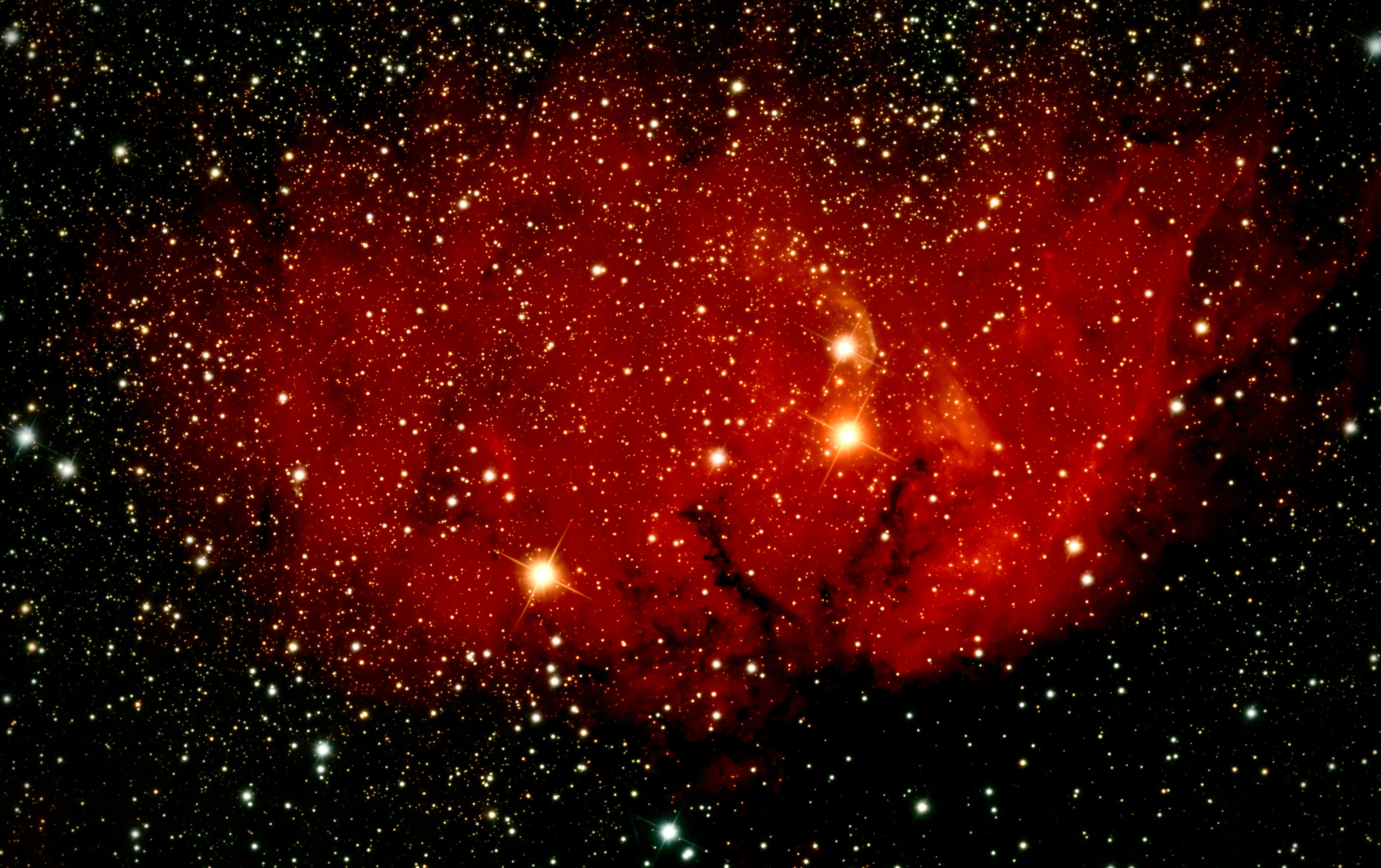
SH2-92 - Emission Nebula in Vulpecula
DISTANCE: ~12,000–14,000 LIGHT YEARS | TYPE: H II REGION
SH2-92 is the ninety-second entry in Stewart Sharpless's 1959 survey of galactic H II regions — vast clouds of interstellar hydrogen ionized by the ultraviolet output of nearby hot stars, glowing as their electrons recombine. Lying in Vulpecula almost exactly in the plane of the Milky Way, it spans over 200 light years, and its ionizing source is believed to be WR 127, a Wolf-Rayet star in the brief, violent phase a massive star enters as it strips away its own outer envelope. Distance estimates place it near the outer edge of the Orion Arm, though they disagree by a couple of thousand light years.
Its sheer size works against it visually: the same emission spread across a degree of sky is a faint wash rather than a bright object, and it is imaged far less often than showpiece nebulae a fraction of its true extent. This portrait took 27.5 hours across nine nights, split between hydrogen-alpha and doubly-ionized oxygen — the red and the teal respectively — and doubles as the first target processed end to end without human intervention. The write-up is in The Science →
On Earth: ~11,000 BC
This light set out as the last ice age was releasing its grip. Ice sheets were retreating across northern Europe and North America, sea levels were beginning the rise that would drown the Bering land bridge, and mammoths, giant ground sloths and sabre-toothed cats were entering their final few millennia. Human hunter-gatherers had reached the southern tip of South America, and in the Fertile Crescent the Natufians were harvesting wild cereals from settled villages — the first hesitant step toward agriculture.
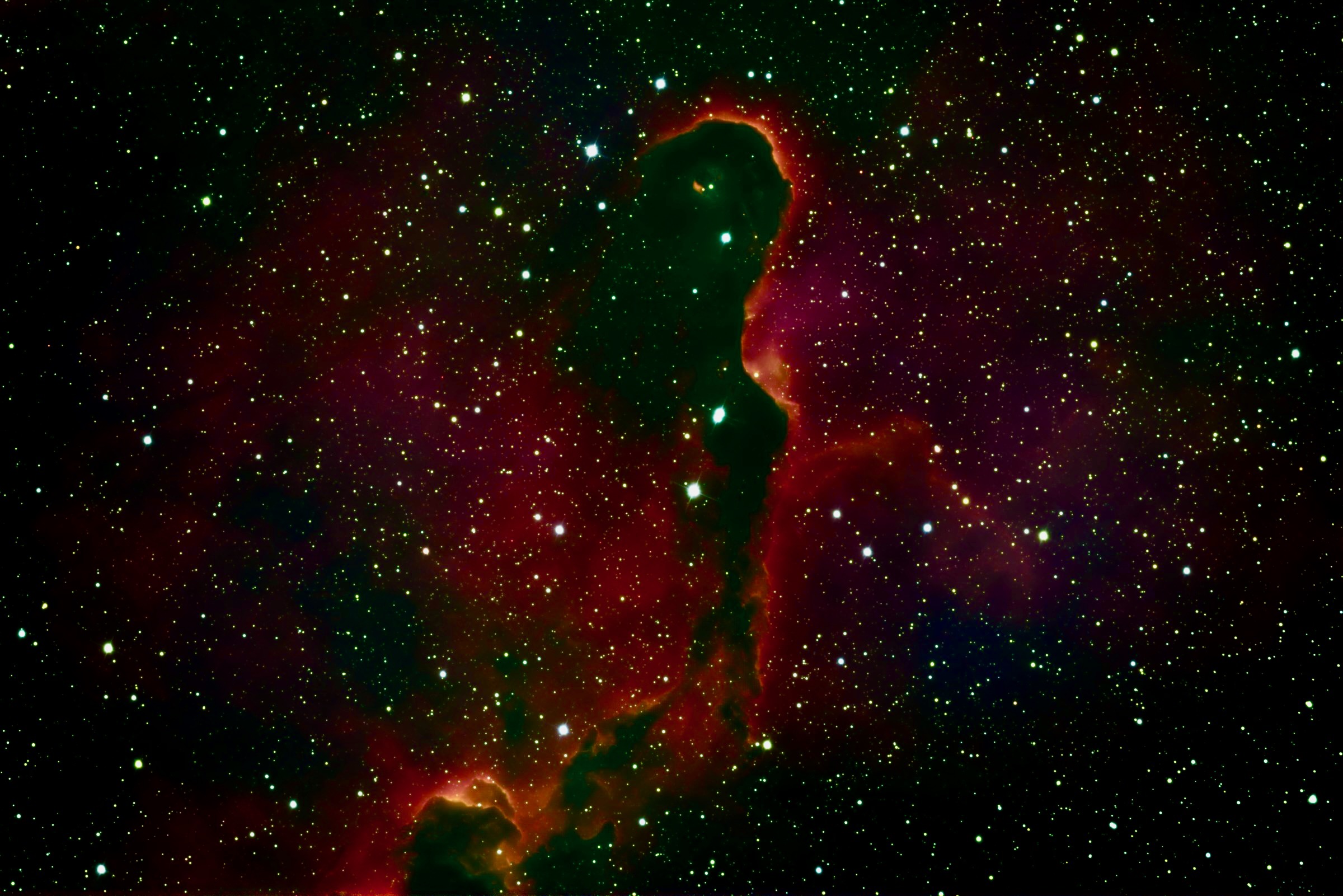
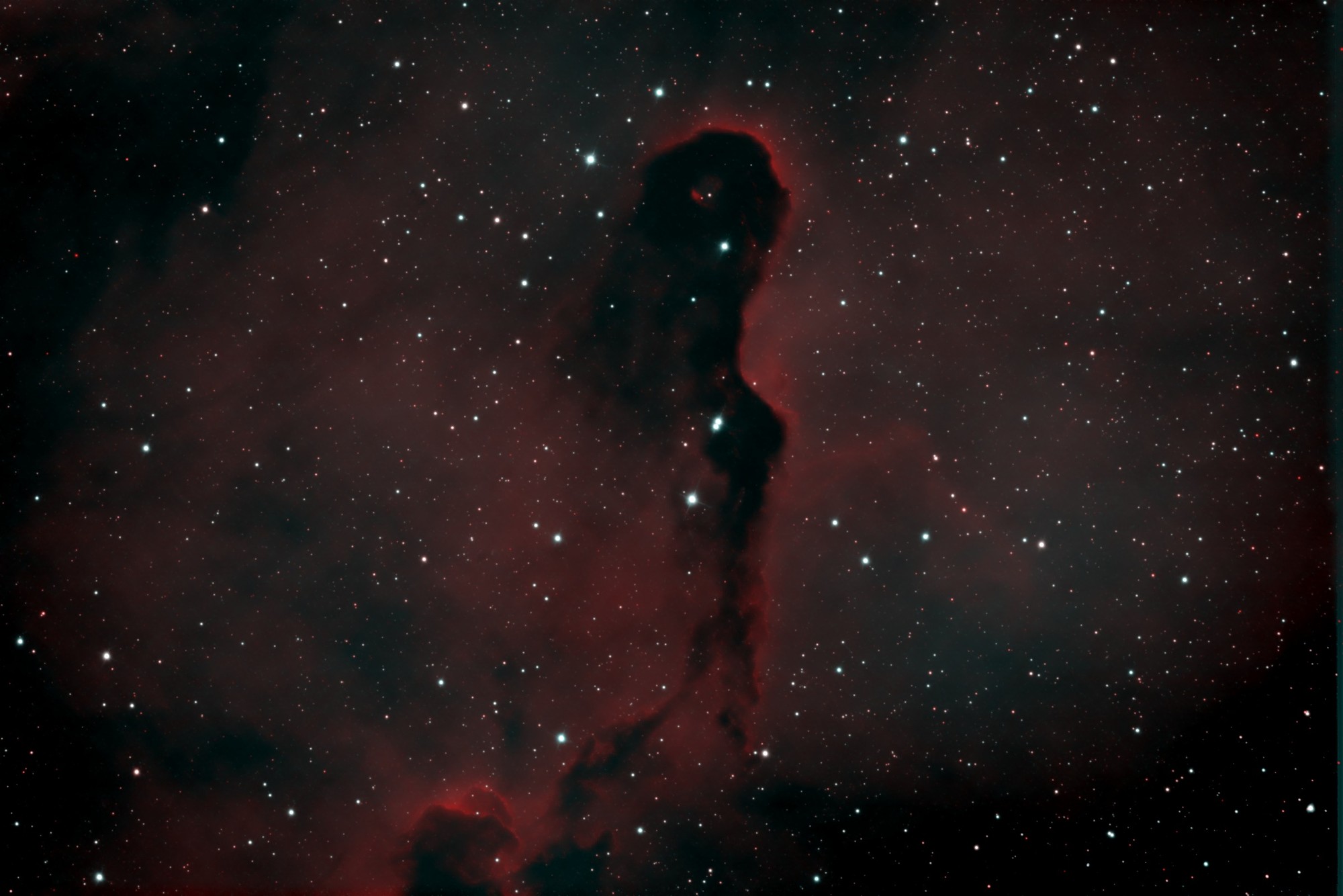
IC 1396A - Elephant's Trunk Nebula
DISTANCE: ~2,400 LIGHT YEARS | TYPE: DARK GLOBULE IN AN H II REGION | 34 Ha + 64 O III + 47 S II × 300 s | 12.1 HOURS OVER FOUR NIGHTS
The Elephant's Trunk is a dense column of cold gas and dust more than
twenty light-years long, hanging inside IC 1396 — a vast
emission region in Cepheus ionized by the hot multiple star
HD 206267, which sits outside this frame. The trunk is what that
star has not yet managed to destroy: its ultraviolet radiation is
boiling material off the column's surface and compressing what remains,
and inside the compressed head a clutch of new stars is forming —
creation triggered by the same radiation that is eating the cloud. The
dark body of the trunk is not an absence of nebula but a silhouette,
an opaque cloud in front of the glowing hydrogen behind it; the case
that such darkness is real absorption, made by measurement rather than
by eye, is in The shadow is the subject.
The colours are a map, not a photograph. This is the HSO
palette: three narrowband filters, each passing a single emission line,
assigned hydrogen-alpha → red,
sulfur (S II) → green,
oxygen (O III) → blue. The broad field renders
red shading toward magenta — hydrogen radiating everywhere, tinted
blue-ward where oxygen's high-excitation emission joins it. The rim of
the trunk burns orange-gold: that is where sulfur's low-ionization line
lights up alongside hydrogen, and it traces the ionization front itself
— the working surface where the star's radiation meets the cloud.
Two of these three lines are fifteen nanometres apart in the deep red,
indistinguishable to the eye, which is why the palette exists at all
— the argument is made in full in
The Crescent in three ionization states.
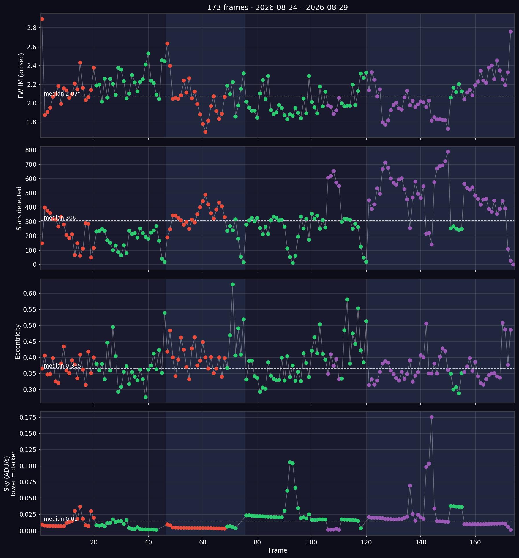
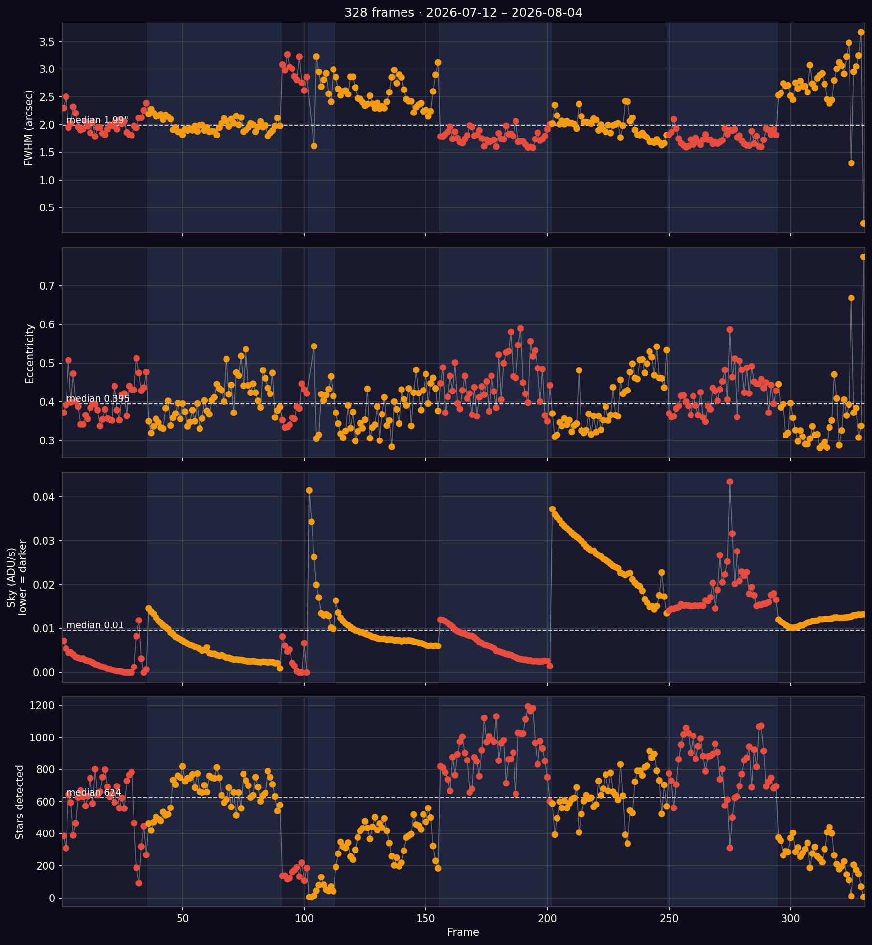
The data behind the picture: 174 five-minute exposures over four nights
(2026-08-23 to 2026-08-28), of which 145 survived the quality gate
— 12.1 hours in the final image. The chart below tracks the four
metrics measured on every frame across those evenings — star
sharpness (FWHM), stars detected, star elongation (eccentricity), and
sky brightness — each dot one exposure, coloured by filter, each
shaded band one night.
Four metrics across the evenings, one dot per frame:
Hα in red, O III in green, S II in purple. The sky
panel shows the moon and haze coming and going; the FWHM panel is
the seeing doing the same.
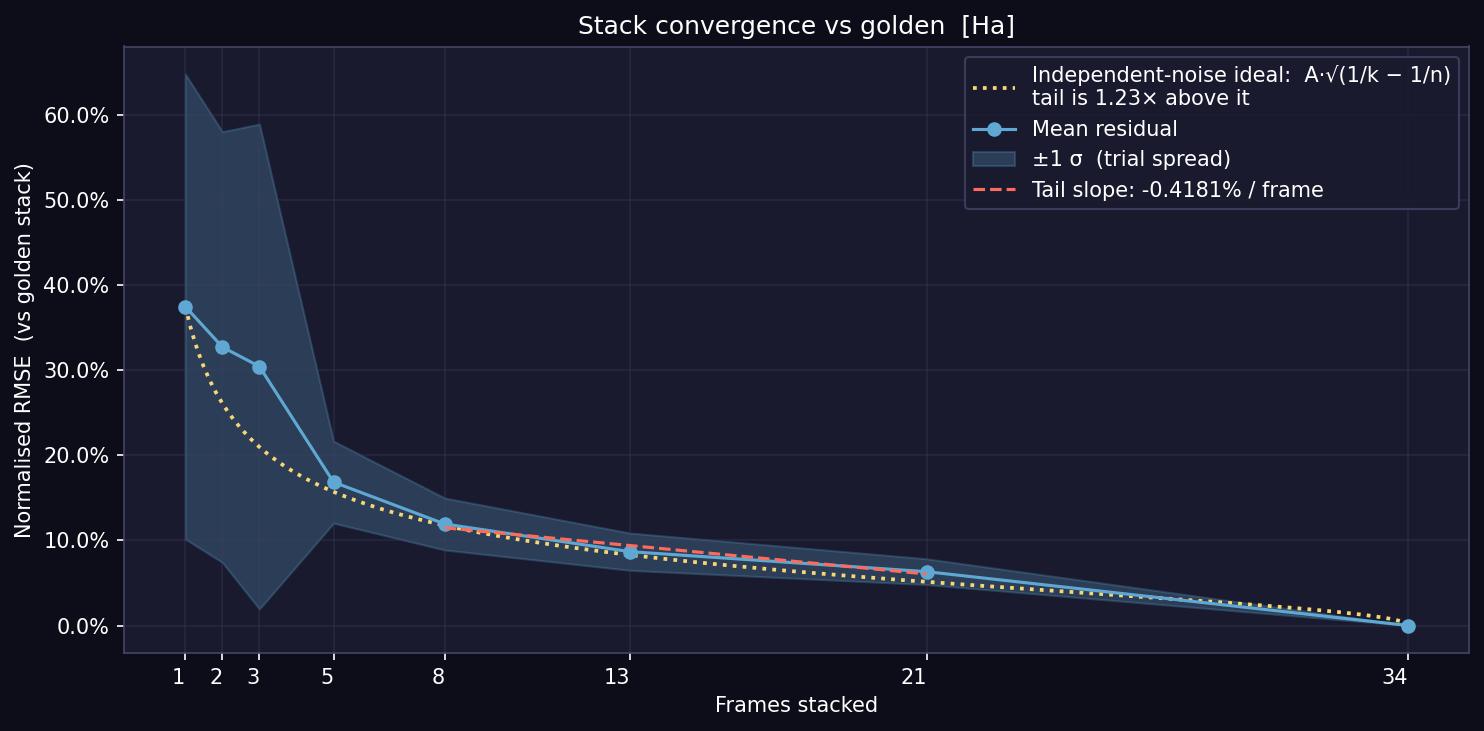
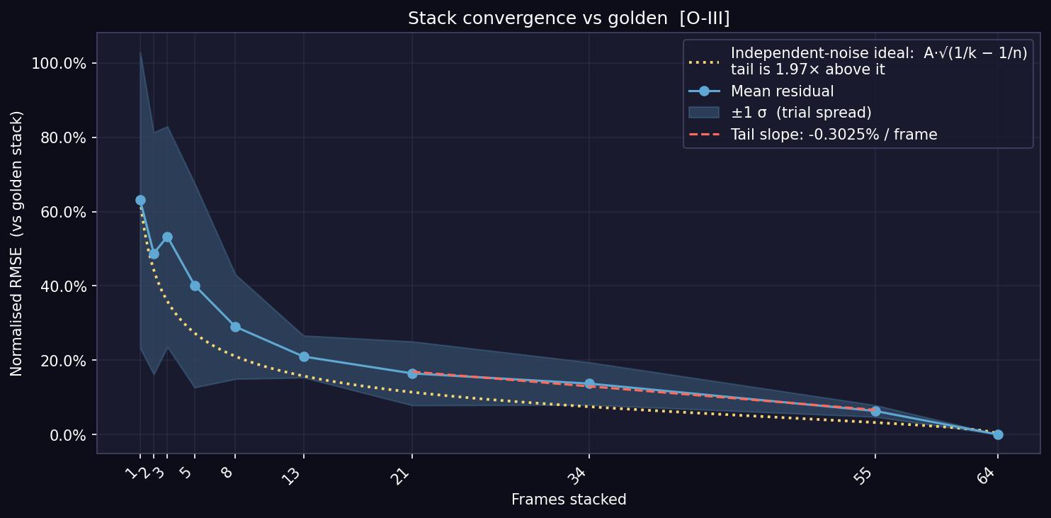
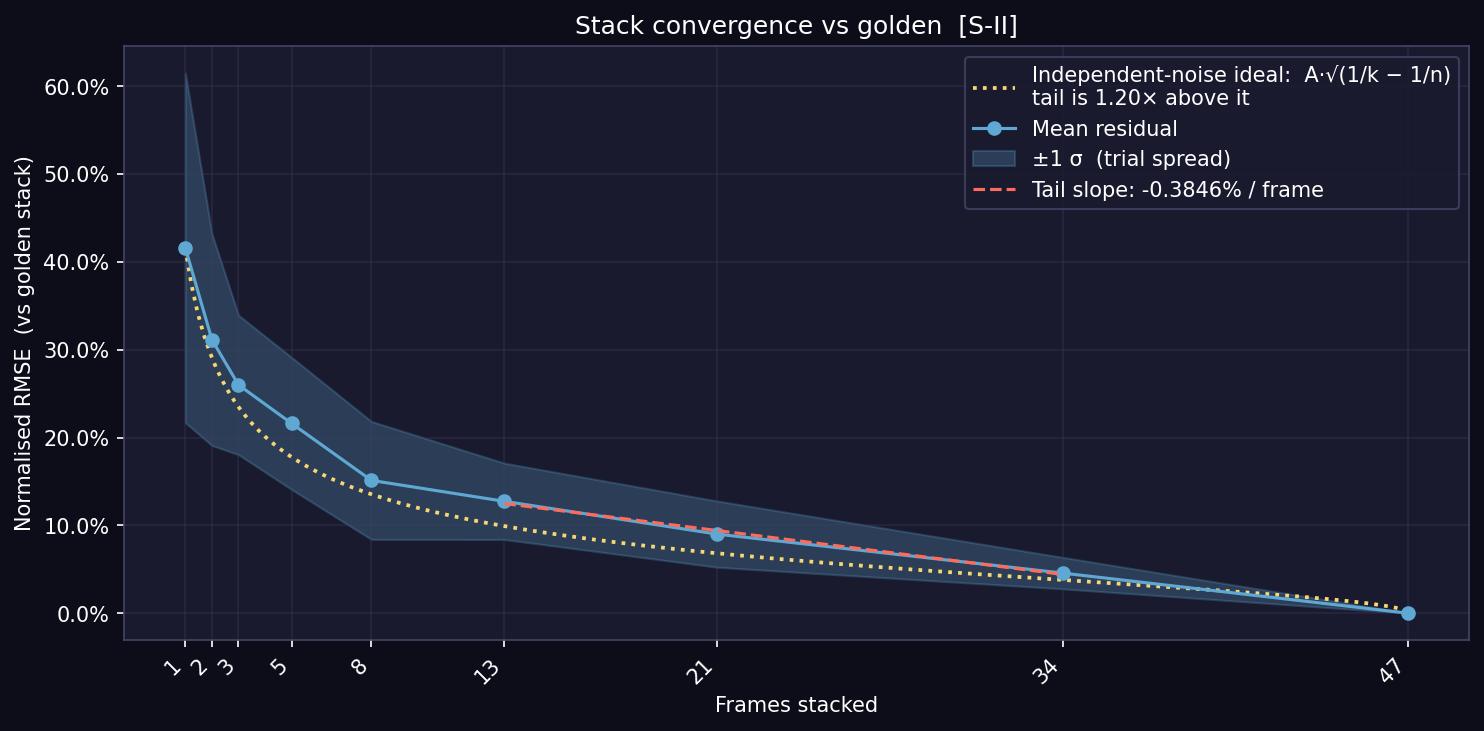
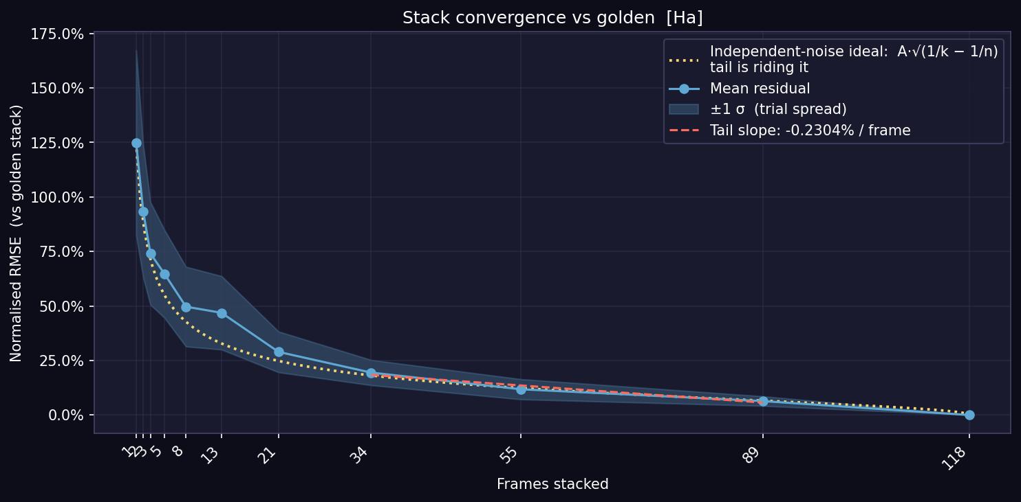
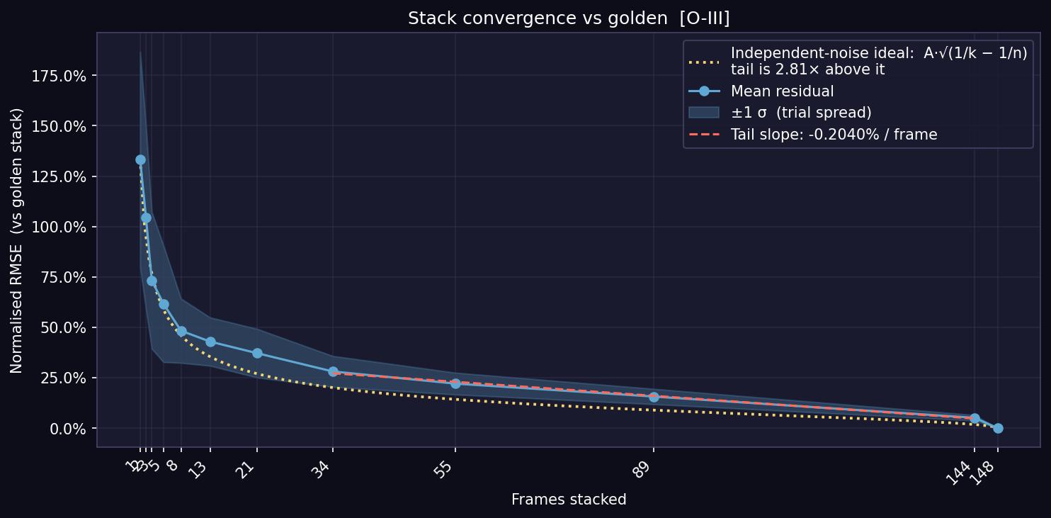
And the question every added frame is supposed to answer: is the stack
still improving? The curves below measure signal-to-noise convergence
per filter — how far a stack of the first k frames sits from the
full stack, as frames accumulate. When the tail flattens, more frames
are polish rather than progress. O III (64 frames) and S II
(47) have flattened below the 0.40 %/frame threshold this
observatory calls converged; Hα, at 34 frames and
−0.42 %/frame, is the one channel still earning its
exposure time.
Hα — 34 frames, tail slope
−0.42 %/frame: still improving.O III — 64 frames,
−0.30 %/frame: converged.S II — 47 frames,
−0.38 %/frame: converged.
On Earth: ~400 BC
This light left during the golden age of classical Greece. Socrates
was questioning his fellow Athenians in the agora — he would
drink the hemlock in 399 BC — and his student Plato would soon
found the Academy. The Parthenon stood newly finished on the
Acropolis. Rome was a young republic still confined to central
Italy; in China the Warring States period was beginning and the
disciples of Confucius were compiling the Analects.
Telling the telescope where focus will be before it looks
2026-09-12 · FOCUS · 580 AUTOFOCUS RUNS, MARCH–SEPTEMBER · TEMPERATURE MODEL PER FILTER · STATUS: BUILT, FIRST NIGHT PENDING
Abstract
Six months of the telescope's own autofocus records show that the focus
position of every filter follows the focuser's temperature along a straight
line — about 80 steps per degree — with only two or three hundred
steps of scatter around it, and that the seven filters sit at fixed
distances from one another. They also show why the autofocus had been
failing: across the whole range it had been sweeping, stars grow by
only 12 percent, less than the noise of a single measurement, so there
was no curve to fit. On the night of 11 September four of six runs failed
and the first O III exposure was taken at the Hα focus, a thousand
steps off. From now on each filter block begins by moving the focuser to
where the model says focus will be at the current temperature, and the
autofocus only refines it. On that night's data the model would have
started 48 steps from the answer.
The night that prompted this
Focusing a telescope is the same job as focusing a camera lens, except that
the "lens" is a 17-inch mirror system whose length changes as the night
cools, and there is nobody at the eyepiece. So the telescope refocuses
itself: it steps the focuser through a range of positions, photographs a
star field at each, measures how big the stars are, and fits a V-shaped
curve to the results. The bottom of the V is focus. It repeats this every
time it changes filter, because the filters are not quite the same
thickness of glass, and every time the temperature drifts a couple of
degrees.
On 11 September the sequence began with thirty-three minutes of autofocus
attempts before it took a single picture. Four runs through the luminance
filter were rejected by the fitting software, then one through Hα,
before a sixth finally passed. Later, at the switch to O III, the run
that was supposed to refocus for the new filter stepped through five
positions, found the stars essentially the same size at all of them, and
gave up. When an autofocus run fails the software puts the focuser back
where it started — which was the Hα focus — and carries on.
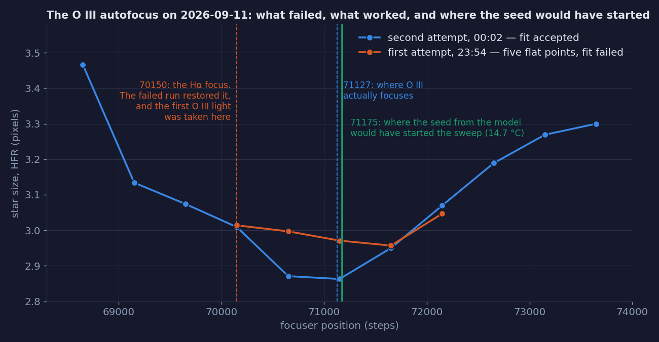
So the first O III exposure of the night was taken a thousand steps from
where O III focuses, and the stars in it were 2.5 arcseconds across
instead of 2.3.
The two O III runs that night. The first attempt (orange) saw
five points that differ by less than the measurement noise and had
nothing to fit; it restored the focuser to 70150, the Hα focus, and
the first exposure was taken there. The second attempt (blue), starting
from the same place but walking further, found the V and put focus at
71127. The green line is where the temperature model, given the
focuser's reading of 14.7 °C, would have started: 71175.
Why the sweep was failing
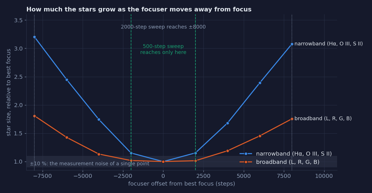
The autofocus was sweeping in steps of 500, four steps either side of its
starting point, so it only ever looked at focuser positions within
±2000 of where it began. The chart below, built from the summer's
accepted runs, shows what that range actually contains on this telescope.
At ±2000 steps the stars have grown by about 12 percent through a
narrowband filter and by almost nothing through a broadband one. The
measurement of a single point, meanwhile, is uncertain by about
10 percent, because the atmosphere is never still and every exposure
catches a slightly different blur. The V the software was asked to fit was
as deep as the noise. That it succeeded as often as it did is a tribute to
the fitting code.
How much the stars grow with defocus, measured from the summer's
runs. The grey band is the noise of one measurement. Between the green
dashed lines is everything a 500-step sweep could see; the dotted lines
are the reach of a 2000-step sweep, where narrowband stars are three
times their focused size and there is an unmistakable curve to
fit.
The cure for that half of the problem is simply a bigger step, and the
sweep is now 2000, so its outer points reach ±8000 where the curve is
deep. But a bigger sweep is only useful if it is centred somewhere near
focus, and that depends on where the focuser is when the run begins. On
11 September it began at the previous filter's focus every time. The
other half of the fix is to start it somewhere better.
What 580 autofocus runs say
Every autofocus run writes a small report: which filter, what temperature
the focuser's sensor read, where the V bottomed out, and how well the
curve fit. The telescope has been keeping these since March without
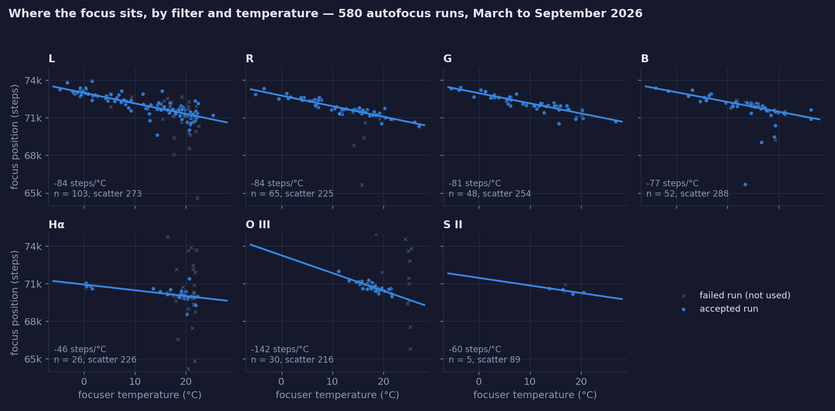
anyone reading them. Plotting the accepted ones — the runs whose fit
the software itself trusted — gives the picture below.
Focus position against focuser temperature for each filter.
Dots are runs the autofocus accepted; crosses are runs it rejected, which
are not used. Each panel's line is the model that now seeds that
filter, with its slope and the scatter of the points about it. The
O III line is steep and rests on a narrow band of temperatures; see
the caveat below.
Three things stand out. The focus moves with temperature at a steady rate:
the broadband filters agree on roughly 80 steps per degree, so a night
that cools from 20 °C to 10 °C carries the focus 800 steps.
The filters are not parfocal, and their offsets are stable: Hα sits
about 1400 steps below luminance, O III about 700, S II about 1300.
And the scatter about each line is 200 to 300 steps, which is about what
a single autofocus run is good for in ordinary seeing; the line is not
worse than a measurement, and it is available before any measurement has
been made. The rejected runs, the crosses, scatter thousands of steps
from the line, which is exactly why they are rejected.
One caveat the plot makes visible. The O III filter has only been
autofocused between 11 and 22 °C, and its fitted slope is nearly twice
the others'. Stretched to a frosty night that line would predict a
position two thousand steps from where the broadband trend would put it.
The model is refitted from the reports every time a sequence is generated,
so the first few cold O III nights will pull it into line; until then the
2000-step sweep has enough reach to absorb the error.
The seed
The mechanism is deliberately small. When the observatory writes the
night's imaging sequence at noon, it now inserts one instruction before
every filter block: move the focuser to slope × temperature +
intercept, using that filter's line, with the temperature read from the
focuser's own sensor at the moment the instruction runs — not a
forecast made at noon. The imaging software already has exactly this
instruction; it only needed the two numbers. The move happens before the
filter changes, so the autofocus that follows the filter change sweeps
around the prediction. And if that run fails, the position it restores
is the prediction, not the previous filter's focus.
The seed does not replace the autofocus. Its scatter, 200 to 300 steps, is
the width of the region the sweep covers anyway; what it removes is the
case where the sweep is centred a thousand steps away and sees only one
arm of the V. The autofocus still has the last word every time, and each
run it accepts becomes one more point on the line.
What to watch
The first exposure of each filter is the test. On 11 September the first
O III frame was measurably softer than the second; after the seed it
should not be. The other number to watch is how many autofocus runs the
software rejects per night, which was four of six. The noon log now records
the seeds it wrote, so a bad night can be traced to the model or to the
sky. As of this note the code is in place and the model is fitted; the
first night that runs with it has not yet happened.
The $25 camera that caught a space station
2026-09-03 · TIANGONG · SECURITY CAMERA AS SATELLITE TRACKER · 1.04°/s · THROUGH CLOUD
Abstract
A cheap outdoor security camera — the kind sold to watch a
driveway — photographed the Chinese space station crossing the sky
above the observatory, unattended, at 20:49 on a night so cloudy the
telescope never opened its roof. Nobody was watching. The camera knew the
station was coming because the observatory had worked out the pass from
orbital data that morning, armed itself, and started recording ninety
seconds before. And we can prove the bright dot in the video is not a star
without knowing a thing about astronomy: it moves 29 pixels every second,
and stars move about 0.004.
How a driveway camera becomes a tracker
The camera is a consumer Wi-Fi model bolted outside the observatory,
pointing up. It exists to answer a much duller question — is it
cloudy? — by counting stars every five minutes. It has no
telescope, no tracking mount, no cooling, and a single one of its pixels
swallows two arcminutes of sky: the full moon, if it wandered into frame,
would be about sixteen pixels across. The telescope thirty feet
away spreads that same moon over seven thousand.
None of that matters for satellites, because a space station is not a
faint thing. The ISS is brighter than every star in the sky and brighter
than most planets; Tiangong is a magnitude or two behind it but still
comfortably in the "you would notice it from a parking lot" category.
What a satellite demands is not sensitivity. It demands knowing
where and when to look, and being awake at 4 in the morning.
Computers are excellent at both.
So the observatory does this. Every day at noon it downloads the current
orbital elements for the ISS and Tiangong — published freely, since
everything in orbit is tracked by radar whether its operators like it or
not — and works out every pass in the next eighteen hours. Then it
throws almost all of them away. A pass only counts if three things line up
at once: the station has to climb above 40° so it is inside the
camera's field rather than behind the trees, it has to be lit by sunlight
on a site that is already dark (satellites are only visible in that narrow
window where they are in daylight and you are not), and it has to stay
that way long enough to film. That trio lines up perhaps a few times a
fortnight. When it does, the observatory writes itself a note, and a job
that runs every five minutes checks that note and spawns a recorder six
minutes before the station arrives.
The one that got away, and the one that didn't
Confession, because it is the more interesting half of the story: this
had been quietly broken since the day it was written. The five-minute job
that checks the note was checking it only in daylight — a
single misplaced indent — and a visible pass is, by definition,
something that happens at night. So the observatory dutifully predicted
passes, armed itself, and then never once looked at its own note at the
moment it mattered. The feature's only successful recording in its entire
life had been a test run in broad daylight: the exception that proved it
could never work. It took a very ordinary question — "did you record
the ISS last night?" — to find it. Thirty-six hours later it caught
a space station.
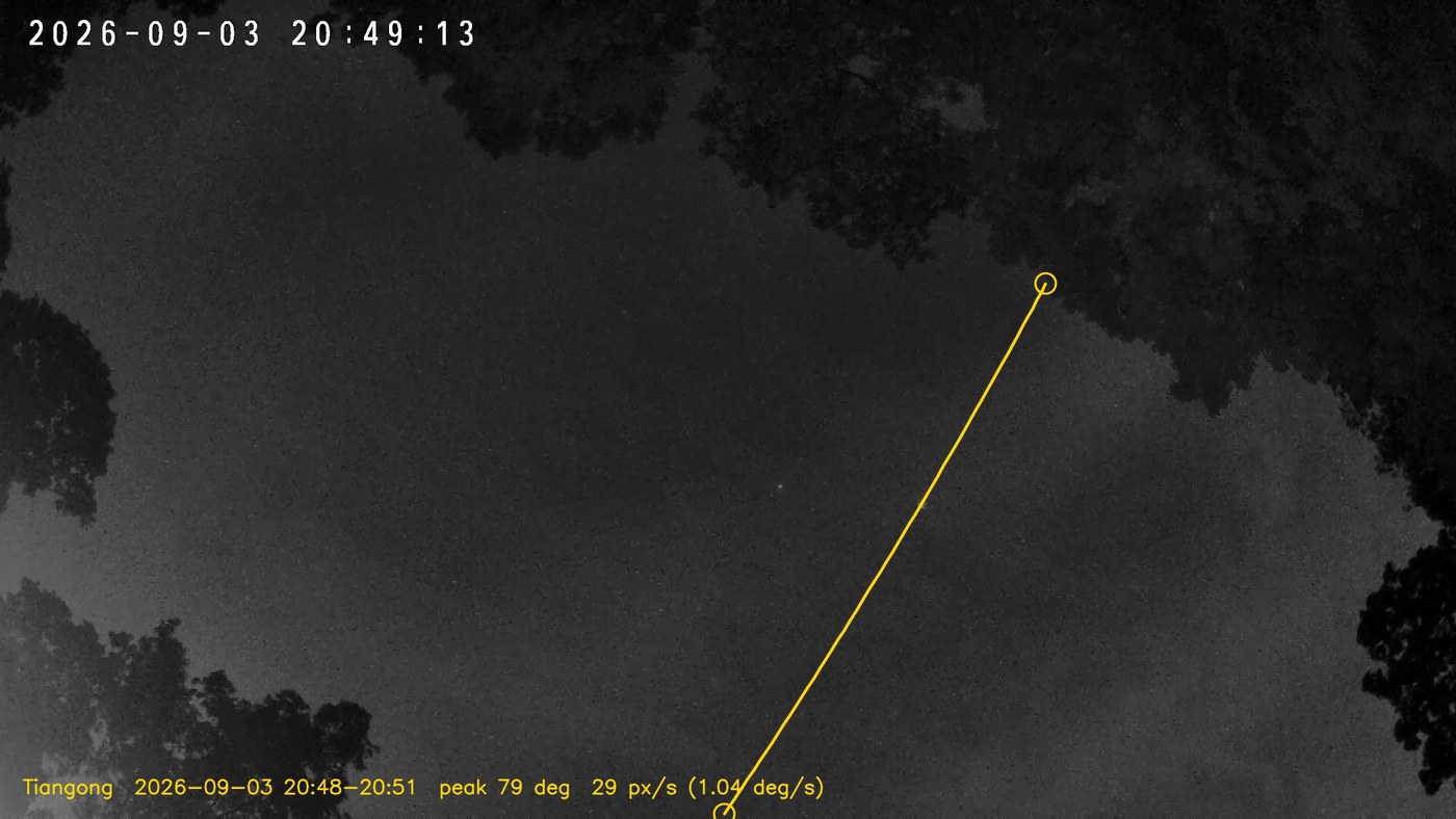
The video
Tiangong, 2026-09-03, 20:49 local. The gold ring follows the
station; the box at top right is the same view magnified 3× so
the dot is actually visible. The timestamp runs in the corner. Those
are the observatory's trees around the edge and, in between, a solid
overcast — the telescope stayed shut all night.
It is filmed through the clouds, not between them
The sky that night was genuinely bad. The camera's own cloud detector
rated the frame untrustworthy at the very moment of the
pass: of 403 things it detected that looked like stars, 163 were measured
to be false — cloud texture masquerading as points of light. The
observatory's plate-solver, which normally matches 122 catalogue stars,
could match 16. By every measure the instrument had of the sky, the sky
was closed for business.
And the station sailed straight through it anyway. That is the part worth
sitting with: a space station is bright enough that thin overcast dims it
without hiding it. So this particular capability — unlike every
other thing the observatory does — is almost weather-proof.
On a night when the serious instrument in the shed — the one with
the carbon fibre, the seven filters and the opinions about seeing
— contributed nothing but a closed roof and a dehumidifier bill,
the security camera on the outside wall got the shot.
Proving it is not a star: pixels per second
A bright dot in a night video proves nothing by itself. Airplanes,
satellites, planets, hot pixels, and reflections off a passing bird all
look about the same in one frame. The distinguishing feature is not
brightness or colour or shape — it is speed, and
the maths is refreshingly blunt.
The sky appears to rotate once a day, so a star drifts across this
camera at about 0.004 pixels per second: over the whole
two-minute recording it moves half a pixel, which is to say it does not
move. The station was measured at 29.2 pixels per second
— more than seven thousand times faster, crossing a quarter of the
sky in the time it takes to read this paragraph. In real units that is
1.04° per second, which is precisely what an object 400 km up and
travelling at 7.7 km/s looks like when it passes nearly overhead. No
identification required: nothing else in the sky moves like that.
Fifty-eight separate detections, one straight line. The gold
track is the path measured across 38 seconds of video; the circles
mark the first and last frames where the station outshone the
cloud.
Finding that line took one small trick, and it is a nice illustration of
why cloudy data is hard. Asking "what is the brightest thing in each
frame?" gives the wrong answer most of the time, because a moonlit cloud
edge is often brighter than a space station. Fitting a line through all
those answers produces confident nonsense. So instead the question is
turned around: which straight, constant-speed path do the most
detections agree with? Clouds cannot conspire to drift in a perfect
line at a constant rate, and satellites cannot do anything else. Out of
260 candidate points across the recording, 58 agreed on a single track and
the rest were weather. One question, correctly posed, does the entire job
of telling a spacecraft from a cloud.
What it costs
Nothing, is the honest answer. The camera was already there counting
stars. The orbital data is free. The prediction takes a couple of seconds
of arithmetic once a day, the recording writes about 25 MB, and old
footage is deleted automatically so the disk cannot fill. The observatory
announces its own catch to the phone in the morning: "Tiangong pass
recorded: peak alt 79 deg at 20:49:22, 2609 frames."
There is something pleasing about the division of labour here. The
expensive instrument in the shed spends months gathering photons from a
nebula that has been sitting in the same place since before there were
people. The cheap camera on the wall waits for something built by humans
to go by overhead at 17,000 miles an hour, and catches it in the rain.
Missing on purpose
2026-08-30 · DITHERING · SIMULATION + SOAP BUBBLE / ELEPHANT TRUNK DATA · STATUS: RA FIX BUILT, AWAITING FIRST NIGHT ON SKY
Abstract
Deliberately adding random pointing errors between exposures — dithering
— makes the final stacked image cleaner, which sounds backwards: the
telescope goes deeper by aiming worse. The reason is that a camera produces two
kinds of noise, and only one of them averages away with more frames. Random
photon noise is different in every frame and falls as √N; hot pixels and
row banding are bolted to the detector and identical in every frame, so stacking
a hundred subs leaves them at full strength. Dithering converts the second kind
into the first. A simulation below shows a held-still stack hitting a hard SNR
ceiling at about a fifth of what the same detector delivers when dithered
— and this observatory's own data shows the ceiling in the wild: a stack
whose SNR grew from 2.7 to only 4.5 between 2 and 29 frames, where √N
promised 10. Chasing that number uncovered a dither that was quietly broken in
one axis, a mount that was wrongly blamed for it, and a trigonometric trap that
made a flawless correction look 45% short.
The wrong intuition, and why it is wrong
The intuition says: point at the target, hold perfectly still, and let the
frames pile up. Every pixel then sees exactly the same patch of sky all night,
the signal adds coherently, and any motion can only smear things. Holding still
feels like discipline. It is actually the one pointing strategy guaranteed to
stop a stack improving.
The √N law — stack N frames and the noise falls by the square root
of N — carries a fine-print clause that everything here hinges on: it
applies only to noise that is independent from frame to frame. Photon
shot noise and read noise qualify; every frame rolls new dice. But a sensor also
carries a fixed pattern — hot pixels, warm columns, row-bias banding,
flat-field residuals — that is the same in every frame, because
it belongs to the silicon rather than the sky. Averaging identical copies of
something reproduces it exactly. Stack ten frames or ten thousand: the random
noise sinks toward the fixed pattern, and then the image stops getting better,
because what remains was never random.
Dithering breaks the symmetry. Shift the pointing by a random handful of pixels
before each sub, then register the frames back onto the stars before combining.
In sky coordinates the target lands in the same place every time — but the
detector's fixed pattern, dragged along by the registration, lands somewhere
different in every frame. From the stack's point of view the pattern
has become one more source of frame-to-frame random noise, and √N applies
to it again. Better still, a hot pixel now visits each sky position only once,
which is exactly the lone-outlier shape that sigma-clipping rejects outright.
Nothing about the detector changed; its noise was merely decorrelated from the
sky.
A controlled demonstration
Real nights never offer a clean A/B — nobody spends five hours
deliberately not dithering — so this one is synthetic, with every noise
source known exactly. A 256-pixel toy detector observes a faint nebula whose
surface brightness peaks at 0.4 σ of a single frame's noise —
genuinely invisible in any one sub. Each frame gets fresh random noise
(10 ADU), plus a fixed pattern that never changes: 90 hot pixels and
row/column banding of about 2 ADU. Two campaigns of 64 frames differ in
exactly one thing: one holds the pointing perfectly still, the other shifts it
randomly by up to ±16 px per frame. Both are registered and combined
with the same 3 σ-clipped mean.
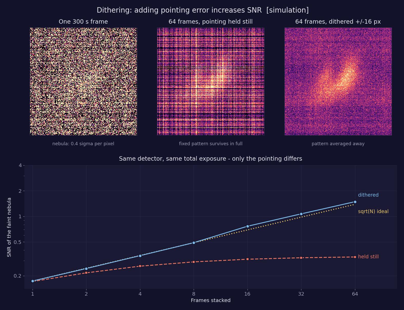
Synthetic data, every parameter known. Left: one frame — the
nebula is nowhere to be seen. Middle: 64 frames stacked with the pointing
held still; the random noise has averaged down, which only exposes the
banding grid and hot pixels underneath, and the nebula is buried in wreckage
that will never average away. Right: the same detector, same exposure,
dithered — the pattern is gone and the nebula simply appears. The
curve underneath is the whole argument in one line: held-still SNR flattens
at 0.33 while the dithered stack tracks the √N ideal to 1.5, and the
gap is still widening at 64 frames. The dithered curve actually edges
above the dotted ideal, because the ideal is anchored to the first
frame's noise, which includes the fixed pattern — and the dithered
stack is removing that too.
The middle panel deserves a second look, because it is the counterintuitive
claim made visible. Those 64 frames are not wasted — their random noise
really did fall by a factor of eight — and that is precisely the problem.
Averaging is a flashlight: it dims everything random and leaves everything
systematic standing, so the cleaner the stack, the more clearly it renders the
detector instead of the sky.
The ceiling, observed on a real telescope
This observatory ran into the ceiling before it had a name for it. On a 50-sub
night on the Soap Bubble field, the stack's SNR grew from 2.69 at 2 frames to
4.53 at 29, where independent noise predicts 10.25. Sub-√N growth is the
signature of noise that does not average down. The dither setting looked
healthy on paper — but measured from the frames themselves, the median
pointing step between consecutive subs was about 3 px against a stellar
FWHM of 6.38 px. A defect moved less than half a star-width between
neighbouring frames: adjacent subs kept landing it on the same piece of sky,
where it stops looking like a lone outlier and starts looking like signal.
Dither that is smaller than a star is barely dither at all.
The pattern being fought is also measurable directly. Differencing consecutive
subs cancels the sky and the nebula and leaves only what changed — and on
the Elephant Trunk data the row means of those differences scatter 7–8×
more than independent pixel noise allows, the column means 6×. That is
real row- and column-correlated banding. (Measured on raw frames
instead of differences the figure comes out a spectacular and bogus
18–23×, because the nebula itself spans whole rows; the measurement
only means something after the sky has been subtracted away.) It also explains
an otherwise puzzling asymmetry: O III stacks converged far worse than
Hα from the same nights — not because O III frames are worse,
but because both filters carry the same banding and O III's signal is
weaker, so the un-averaged residue is a larger fraction of it.
The bug, the false accusation, and the cosine
Fixing the amplitude was supposed to be the end of the story: raise the dither
to 20 px and move on. The next run's FITS headers said otherwise. Dec was
dithering beautifully — rms 11.8–14.5 px, right on target. RA:
0.1 px. One axis of the dither simply was not happening, and a 1-D dither
is a line on the sky — it averages one banding family and leaves the
perpendicular one untouched, forever.
The sequencing software's own log showed it commanding both axes correctly, so
suspicion fell on the mount: perhaps a direct-drive servo holding to its
tracking model treats an RA rate-pulse as an error to be corrected, and quietly
nulls it. A live test settled it — command the mount's native offset API
to move +30 arcsec in RA and watch what sticks. The answer came back
16.4 arcsec, and for a moment that read as the mount complying with 55% of
the request. It is nothing of the sort: the command is in RA-coordinate arcsec,
the measurement is on-sky arcsec, and at declination 56.9° they differ by
exactly cos(dec) = 0.547. The offset held to a ratio of 0.9999. The
mount was flawless; the arithmetic reading the test was where the bug nearly
landed. Read the raw numbers side by side and a perfect mount looks like a
broken one — the opposite of the truth.
So the fault is in the pulse-guide path the sequencer uses to nudge the mount,
not in the mount itself — the pulses go out and the servo tracks straight
back. The fix routes around it: a script dithers through the mount's offset API
directly, with the sequencer still deciding when. Offsets are set
absolutely rather than accumulated, so a missed call cannot compound into a walk
off target, and the RA amplitude is divided by cos(dec) up front — the
cosine that mislabelled the mount now sized into the command where it belongs.
Simulated over 400 dithers it delivers rms 11.9 / 11.6 px on both
axes. The number that will prove it on sky is a single statistic in the next
run's FITS headers: RA rms ≥ 8 px. As of this note, that night has
not yet happened.
What settled out as practice
Dither every sub, not every few — rejection works because a defect is a
lone outlier at its sky position, and three consecutive hits stop being an
outlier. Size the step to roughly three times the stellar FWHM: below one FWHM
it buys little (as measured above), beyond five it just spends settle time. The
cost of all this deliberate imprecision, measured across a real night, is about
12 seconds per 300-second sub — four percent — and that covers
readout, download, the move and the settle combined. Four percent of the night,
paid to make the other ninety-six actually accumulate.
The general lesson is the one this series keeps re-learning in different
costumes: more data only helps with noise that differs from frame to frame, so
the first question about any noise source is not "how big is it?" but "does it
repeat?" Whatever repeats must be made to stop repeating — calibrate it
out, or scramble its relationship to the signal — because no quantity of
averaging will touch it. Dithering is that scrambling, applied with a
telescope. The pointing errors were there all along; the only change is that
now they are large, random, and working for us.
The shadow is the subject
2026-08-24 · IC 1396A, THE ELEPHANT TRUNK · Hα / O III · NOISE2NOISE, POOLED NARROWBAND · STATUS: DISPLAY ONLY
Abstract
A night on the Elephant Trunk, stacked and denoised without a human in the loop and
delivered to a phone as a push notification before breakfast. The picture's most
striking feature is the thing that is not there: a black channel winding down the
middle of a red field, with stars showing through it. That darkness is not missing
data and not a failure of the processing. It is a cloud of dust, thick enough to
block the nebula behind it, and it can be shown to be real by measurement rather
than by eye — the dark region reads below the surrounding sky, which
nothing but absorption can do.
The picture
IC 1396A on the night of 2026-08-23, composed as HOO:
Hα → red, O III → green and blue. 14 accepted Hα
frames and 21 accepted O III frames at 300 s each, stacked onto a
single shared reference and denoised after stacking.
What the dark lane is
The Elephant Trunk is a cometary globule — a dense knot of dust and molecular
gas, compressed and sculpted by the ultraviolet light of a hot star outside this
frame. It sits in front of the wider IC 1396 emission region. So the
arrangement is layered: hydrogen glowing across the background, an opaque cloud
between it and the telescope, and the cloud's silhouette is what the camera records.
The picture is not showing a hole in the nebula. It is showing a shadow.
Dust does this because it is very good at stopping starlight. Grains a fraction of a
micron across absorb and scatter optical photons far out of proportion to their
mass, so a cloud that is diffuse by any terrestrial standard is functionally solid
at these wavelengths. What gets through is what was never behind the cloud in the
first place.
How we know it is dust and not a processing artefact
A black region in an astronomical image is exactly the kind of feature that ought to
be distrusted, because there are several dull ways to manufacture one. A stretch
whose black point is set too high will clip faint signal to nothing. A denoiser that
is over-suppressing will flatten low-signal regions toward zero. Both would produce
something that looks like this, and neither would be the sky.
The discriminator is the sign. Clipping and over-suppression can drive a region down
to the sky level; neither can push it below. Absorption can, because
a cloud in the foreground removes light that the surrounding sky still delivers.
Measured on the raw stacks against a single global sky value — no
two-dimensional background model, so nothing in the fitting could absorb the nebula
— the darkest tiles come out at −2.74 ADU in
Hα and −2.00 ADU in O III, against
sky levels of 4.26 and 2.62. Averaged over a 128-pixel tile the noise on that
measurement is 0.012 ADU, which puts the deficit at more than
200 standard deviations. It is not noise, and it is not the
floor of the stretch.
A second, independent check comes free with narrowband. The two filters were stacked
separately, from different frames, and they darken by similar amounts in the same
places — Hα by 1.75 σ and O III by 1.62 σ
relative to their own skies, over the same span of the frame. Extinction by dust is
broadly achromatic across two lines this close together, so that agreement is what
the physics predicts. A processing fault would have no reason to land in the same
place, at the same depth, in two channels that never saw each other.
The stars scattered across the dark lane are consistent with the same picture rather
than a contradiction of it. Most of them lie in front of the globule, between it and
the telescope, so nothing dims them; a few are background stars seen through thinner
material at the cloud's edges. In the darkest tiles the globule is removing roughly
60% of the Hα signal that reaches the sky around it, which is why it renders as
flat black once stretched.
The denoiser, and the notification
The image was produced by the observatory's Noise2Noise model, which is trained
without any clean reference at all: it learns from pairs of independent stacks of the
same field, where the only difference between the two is the noise. This particular
model was pooled across Hα and O III and trained on a different object
entirely — it had never seen the Elephant Trunk. It is applied once, after
stacking rather than to each frame, which costs about eleven seconds per channel and
cannot launder a shared bias into an apparently converging result.
The standing rule for this series applies here too, and it is not a formality. The
denoised frame preserves source flux to within a few percent — measured on this
field at 104–117% across every brightness level, faintest included — but
"within a few percent" is not good enough to measure with. The denoised image is for
looking at. Every number quoted above, including the depth of the shadow, was taken
from the calibrated linear stacks, never from the picture.
The whole sequence runs unattended. A scheduled job each morning finds the targets
that gained frames overnight, builds a shared reference, stacks each filter onto it,
applies the quality gate, denoises, composes the colour image, and writes the
products alongside the night's data. The finished denoised composite is then sent
straight to a phone as a push notification, captioned with how many frames each
filter contributed and how many survived the gate — on this night, 14 of 20 in
Hα and 21 of 26 in O III. The first look at the Elephant Trunk was on a
phone screen, several hours after the roof had already closed.
One caveat worth recording, because it nearly produced a wrong conclusion. The
morning's first automatic render set its black point as a percentile of the image's
own pixel distribution. On a denoised frame that rule misfires: removing the noise
narrows the distribution, so the same percentile lands at a different brightness, and
the black point ended up sitting inside the noise. Faint nebulosity that
survives in the raw frame — where random scatter lifts sky pixels above the
cut — fell below it once the scatter was gone, and the denoiser appeared to
have eaten the outer nebula. It had not; the flux was measurably still there. The
fix was to anchor the black point to the measured sky rather than to a percentile.
The lesson is the usual one in this work: a processing choice that is harmless on a
noisy image can become destructive on a clean one, and the failure looks exactly like
a discovery.
The Crescent in three ionization states
2026-08-23 · NGC 6888, CRESCENT NEBULA · Hα / S II / O III · NOISE2NOISE REPROCESS · STATUS: DISPLAY ONLY
Abstract
A reprocessing of this observatory's existing Crescent Nebula data through the
latest Noise2Noise model, rendered in an unusual palette: HSO, with hydrogen
mapped to red, sulfur to green, and oxygen to blue. The palette is the point.
Two of these three emission lines sit fifteen nanometres apart in the deep red,
where the eye cannot tell them apart at all — a narrowband image is not a
photograph of what the nebula looks like, it is a map of which atoms are
radiating where, and false colour is the only way to draw that map. The other
finding is about the denoiser: after many model variants, they all land within
sight of each other. The lever that remains is not architecture. It is
integration time.
The picture
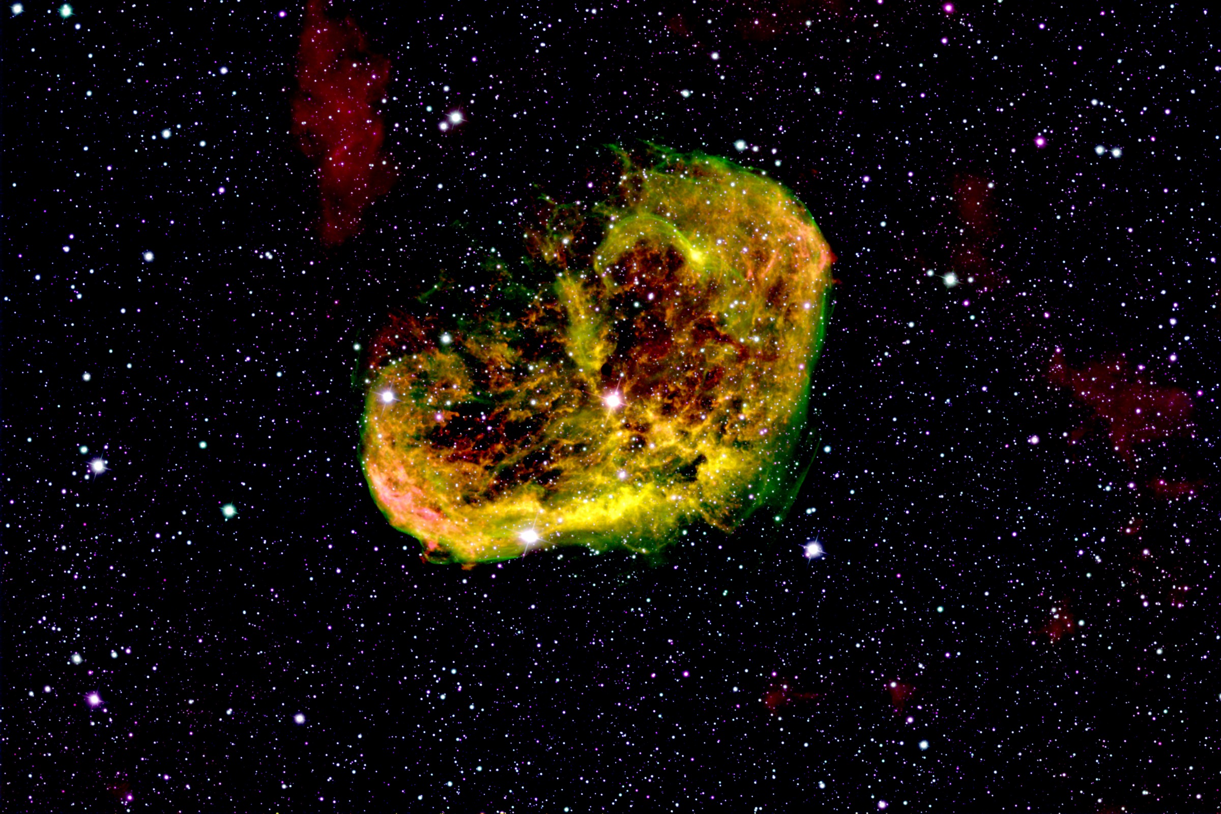
NGC 6888 reprocessed through the current Noise2Noise model
and composed as HSO: Hα → red, S II → green,
O III → blue. The same object, from the same data era as
the gallery's Crescent.
The Crescent is a wind-blown bubble: the Wolf-Rayet star WR 136 spent its
red-giant phase shedding a slow envelope, and now its fast wind is slamming
into that older shell from the inside. Read through the palette, the picture
separates the players. The body of the shell renders yellow — red plus
green, hydrogen and sulfur radiating together in the swept-up ejecta. The
sharp green skin is where S II dominates: the shocked interface itself,
sulfur's low-ionization lines lighting up exactly along the collision front.
The diffuse red patches framing the field are plain hydrogen — the
Cygnus background that surrounds everything in this part of the sky,
radiating Hα with no sulfur to speak of. Where all three lines emit
together, the mix tends toward white.
Fifteen nanometres
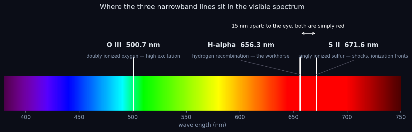
Where the three lines fall. O III sits alone in the
blue-green; Hα and S II are 15 nm apart in the deep red
— indistinguishable to the eye.
Each line is a fingerprint of one atom in one state. Hα
(656.3 nm) is hydrogen recombining after ionization — the
workhorse line, radiated by essentially any gas a hot star has touched, which
is why it traces the bulk of every nebula. S II
(671.6 nm) is singly ionized sulfur, easy to make and easy to
destroy: it survives only in low-ionization gas, which concentrates it at
shock fronts and ionization boundaries — edges, skins, rims.
O III (500.7 nm) is doubly ionized oxygen, which
takes serious ultraviolet or shock energy to produce; it marks the
highest-excitation gas, nearest the star or hottest parts of the front.
Now the problem the chart makes visible: two of those three diagnostics are
both, to a human eye, simply red. Photograph the Crescent in "true colour"
and the hydrogen story and the sulfur story land on the same retinal cells;
the physics distinction is real but invisible. Assigning the lines to three
well-separated display channels is what makes the distinction visible at all
— the green rim on this image is the shock front, as a thing
you can point at. A narrowband palette is routinely criticised for not being
what the object "really looks like". That is true, and it is not the goal.
No emission nebula looks like much of anything to the eye — too faint,
colour vision not engaged. The palette trades a fictional realism for a real
map: which atom, in which state, where.
The denoiser, and where that work has landed
The render was denoised by the latest of the Noise2Noise models this
observatory has been training since the first
result worth showing (the method itself is described in
the original note). The synopsis of the many
variants built since — per-filter models, pooled training, different
losses and normalisations — is easy to state: they all come out very
similar. Once the early bugs were fixed, the architecture stopped being the
thing that mattered; every reasonable variant recovers about the same image
from the same data, because they are all estimating the same signal from the
same photons.
That is a useful negative result. It says the model is no longer the
bottleneck — the photons are. Better pictures now mean more
integration time on the sky, not more epochs on the GPU. The denoiser's
place in the pipeline is settled and modest: a display-stage tool, applied
after the science products are made, never before. As with every image in
this series: the denoised frame is for looking at. Nothing is measured
from it.
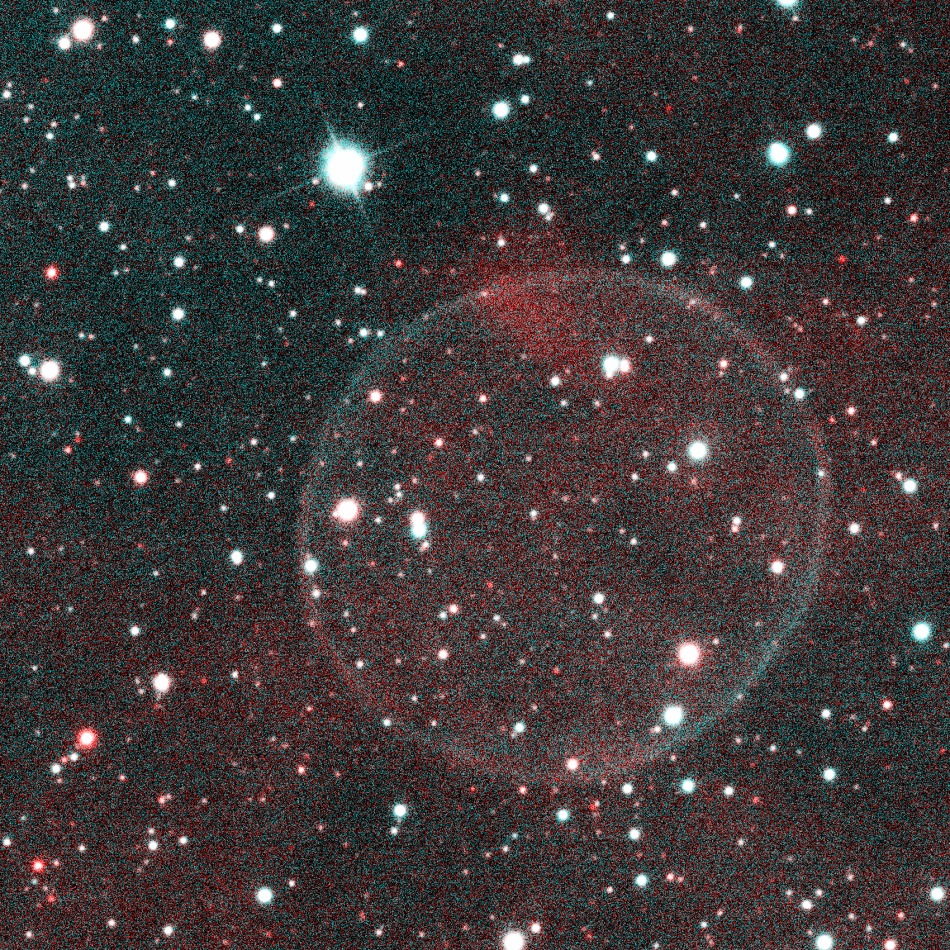
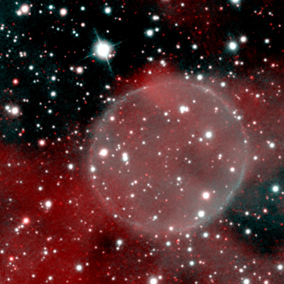
The first denoise worth showing, and why nothing may be measured from it
2026-08-17 · SOAP BUBBLE, PN G75.5+1.7 · O III 500.7 nm, 77 SUBS · HELD-OUT TARGET · STATUS: DISPLAY ONLY
Abstract
The Noise2Noise network trained here has produced its first result that clearly beats the stack it was given. In 77 O III subs of the Soap Bubble the shell is traceable all the way round but no brighter than the grain it sits in; after denoising it reads as a continuous rim with structure along it, and the stars stay round and in place — 93% of the brightest 250 survive, with a median centroid shift of 0.26 px. That last number is the check that matters. The network had never seen this object during training, so this is generalisation and not memorisation. It is also, permanently, not a measurement: a denoiser outputs what was probably there, not what was there, and it removes the visible evidence of uncertainty without removing any of the uncertainty. The output is for looking at. Nothing is computed from it.
The result
The finished frame. Hα red, O III teal; the Soap
Bubble is the small pale sphere at centre, an almost perfect circle
against the Hα clouds of the Cygnus complex. The crops below are
taken from the sphere itself.
Before. The ordinary stack, 1:1. The ring is
there — traceable all the way round — but it is competing
with grain of its own amplitude.After. The same pixels through the network.
The grain goes, the rim holds together, and the stars stay where they
were.
The Soap Bubble is a hard target for this. It is a planetary nebula whose
shell is a thin spherical shock, most of it fainter than the sky it sits
against, and O III at 500.7 nm is where it shows at all. The
denoising was done on that O III channel; the crops are shown in the
same Hα/O III rendering as the wide frame, which is why the sphere
reads pale against red rather than as a bare monochrome ring.
Seventy-seven subs is a real night’s work, and the ordinary stack still
leaves the shell at roughly the amplitude of its own noise — a ring you
can trace, but only once you know to look. In the denoised frame the rim
holds together and varies visibly along its length.
That is the first output from this network that is straightforwardly better
than what went in, rather than merely different from it.
Why the stars are the interesting part
The failure modes here are not subtle, and they appear in the stars before
anywhere else. A network that has learned the wrong lesson eats them: a
point source that lands in a slightly different place in every dithered
frame looks exactly like noise, and a carelessly trained denoiser removes
it. Others smear stars into ellipses, shift them, or keep the bright ones
while dissolving the faint ones — which quietly rewrites the
photometry of the whole field.
None of that happens here. Measured on the two frames above, the count of
real sources goes up rather than down — 314 to 330, as faint
stars climb out of the grain that was hiding them — and of the 250
brightest in the raw crop, 232 survive with a median centroid shift of
0.26 px and 95% inside 0.66 px. Those figures come from the
display-stretched crops rather than the linear data, so they are a sanity
check and not photometry; but a network that ate, smeared or shifted stars
could not produce them. That is the evidence that the network learned
something about this camera’s noise rather than something
about this camera’s pictures.
Held out, which is what makes it a result
The network was never shown a frame of this object. Had it been trained on
Soap Bubble data, a beautiful Soap Bubble output would prove very little
— a large network can memorise, and reproducing a shell it has already
been taught is not the same as recovering one. Evaluating only on targets
held out of training is the difference between a demonstration and an
anecdote, and it is a discipline this project imposed on itself after
an earlier episode where a search that found nothing
looked exactly like a search that worked.
How the training works, briefly
The full treatment is in the earlier note on learning
to denoise without ever seeing a clean image. In short: no clean image of
a nebula exists anywhere to train against, so supervised denoising is
unavailable. Noise2Noise sidesteps the problem by training the network to map
one noisy frame onto another noisy frame of the same scene. The
predictor that minimises squared error against a random target is that
target’s mean; the noise is zero-mean and independent between frames;
so the network converges on the clean signal without ever being shown one. An
observatory that takes hundreds of subs of the same field is close to the
ideal case for it.
Reaching this point took fixing three faults found on 2026-08-11 —
registration against a global reference, a normalisation mismatch between
training and inference, and a BatchNorm problem — together with changes
to the training itself. The earlier outputs were not marginally worse than
this one; they were wrong in ways that became obvious as soon as the stars
were examined.
The part that does not go away
A denoiser does not recover the photons. That information was destroyed when
the noise was added, and nothing downstream restores it. What the network
outputs is an estimate of what was most likely there, given this
input and everything it learned from every other frame it saw in training.
That is a statement about a population. It is not a measurement of this
object.
The consequence is sharper than “it might be wrong”. Grain in an
image is not merely ugly; it is the honest, visible record of how much is
known. Denoising removes that record without removing any of the
underlying uncertainty. The smooth image looks far more certain than the
data behind it is, and it looks that way to a careful reader as much as to a
careless one. That is what makes it dangerous in a way a noisy image is not.
A network minimising expected error will also, handed pure noise, produce
whatever structure is most plausible — because plausible structure is
precisely what minimises expected error. It will hand you a filament that was
never there, and it will look like the filaments that were. The reason to
trust this ring is that the whole circumference is already present in
the raw stack, faintly: the network made an existing feature legible rather
than inventing one. That is a weaker claim than it sounds — it is the
reason to trust this ring, not a general licence — and it is checkable
only because the before frame was kept. Had the ring emerged from a blank field, the correct reaction
would have been alarm rather than pleasure.
What it may be used for
Looking at. Gallery images, presentation, showing somebody what is out there.
That is a real use, and this result is good enough for it.
Nothing else. No photometry — flux is not conserved in any way that can
be trusted. No detections, since a transient search run on denoised frames
would be searching a network’s expectations rather than the sky. No line
ratios, no surface-brightness profiles, no rotation curves, no transit depths.
Every measurement this observatory makes runs on the ordinary stack, and the
denoised frame is a picture made from it afterwards. The stack is the science
product; this is the photograph.
Strands in the stack: a feature that was never unusual
2026-08-10 · SOAP BUBBLE FIELD · 20 Ha + 29 O-III × 300 s · 20th OF 387 SUCH FEATURES
Reservation recorded by the observatory’s owner.
I am not as confident as this analysis is that a software or an optical
cause has been excluded. The conclusions below should be read with that
reservation standing.
The reservation is well founded, and it is worth setting out the grounds
rather than leaving it as a difference of opinion. Every exclusion in this
note was computed by this observatory’s own bespoke pipeline, or by
analysis scripts written alongside it during the investigation, and
several of those scripts returned demonstrably wrong numbers on the way
— a registration measurement that reported no dithering when the
mount dithers every exposure, and a displacement measurement that
contradicted the images it was measuring. The optical exclusions in
particular rest on drift and registration geometry derived from that same
software, so they are not independent of the tool that produced them. The
independent reduction which does not show the feature is
attributed here to a gentler stretch, and that is an assumption rather
than a measurement. None of this overturns the tests below, but a reader
should weigh them knowing that the instrument, the pipeline and the
analysis share an author.
Abstract
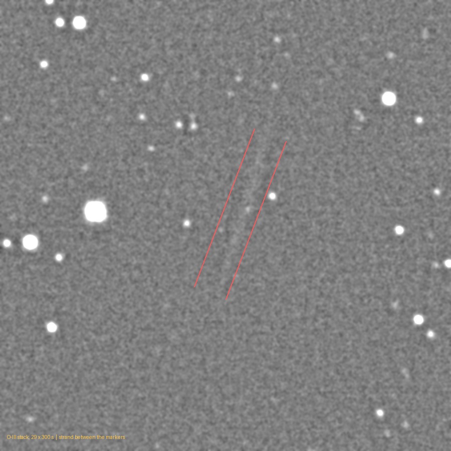
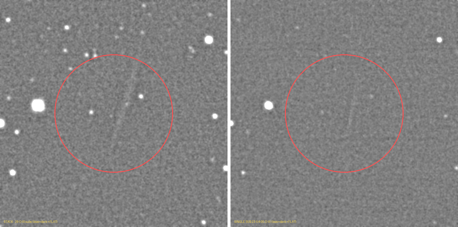
A faint linear feature roughly 55″ long and 5″ wide appears in
deep stacks of the Soap Bubble field, at the same sky position and
position angle in both the Hα and the O III channels. A long
sequence of tests established what it is not: it is fixed with respect to
the stars rather than the sensor, which excludes the optics, the detector
and dust or a chip in the optical path; it survives a median of thirty
frames, which excludes a satellite or meteor; its signal-to-noise
rises with the number of frames combined, which excludes an
asteroid or comet, because stacking dilutes anything that moves; and a
stack of 63 bright stars shows the telescope produces no diffraction
spikes at all. Each exclusion held. The conclusion drawn from them did
not, because one question had never been asked: how many
comparable features does the frame contain? A matched-filter
search finds 387 above 4σ, and the strand ranks twentieth —
the 95th percentile of an ordinary population, not an outlier. The one
measurement that appeared to show the feature varying with time turned out
to be tracking the sky background, which fell 48% through each filter
block and reset at the filter change (r = −0.705). In a field this
dense with filamentary Hα and O III emission the most
economical reading is that it is faint nebulosity, which fits every
established fact without strain. This note is therefore mostly a record of
a methodological failure: excluding exotic explanations one at a time for
a feature whose ordinariness a single measurement would have shown at the
outset.
The observation
The data are a single night, 2026-08-08, on the Soap
Bubble Nebula (PN G75.5+1.7, a planetary nebula in Cygnus; referred
to as “bubble” in this observatory's target list, and not to
be confused with NGC 7635, the Bubble Nebula, which lies 43°
away in Cassiopeia). The field centre is RA
20h15m22s, Dec
+38°02′58″. Twenty 300-second Hα exposures from
21:34 to 23:13 local, then thirty 300-second O III exposures from
23:28 to 02:07, of which twenty-nine were stacked — 4 hours 5
minutes of integration in total. CDK17 at f/6.8, QHY600M,
0.2639″/px.
One night is the single most important caveat on everything below.
Four hours is a short exposure for a target of this surface brightness,
and the feature under discussion sits close to the noise as a direct
consequence. Several of the errors recorded at the end of this note are
errors of reading structure into data that did not have the
signal-to-noise to support it. A second night would change the
arithmetic more than any amount of reanalysis of this one.
The rendering is HOO, a two-filter narrowband palette.
Rather than record red, green and blue, the telescope images through two
narrow filters isolating single emission lines: hydrogen-alpha at
656.3 nm, emitted by ionised hydrogen, and doubly-ionised oxygen at
500.7 nm. The Hα frame is mapped to the red channel and the
O III frame to both green and blue, which is where the name
comes from — H, O, O. Oxygen therefore renders as cyan rather than
green, and the colours in the image are a map of which gas is emitting
where, not what the eye would see. The practical reason for narrowband
is that a 3 nm filter rejects essentially all moonlight and light
pollution while passing the line, so a nebula can be recorded on nights
that would be useless for broadband work.
All stacking, calibration and colour processing here was done locally in
Python — registration, sigma-clipped combination, background
modelling and the stretch — rather than in commercial astronomy
software. That matters for this note only in that every intermediate
product was available for inspection, which is what made the substitution
tests in the next section possible.
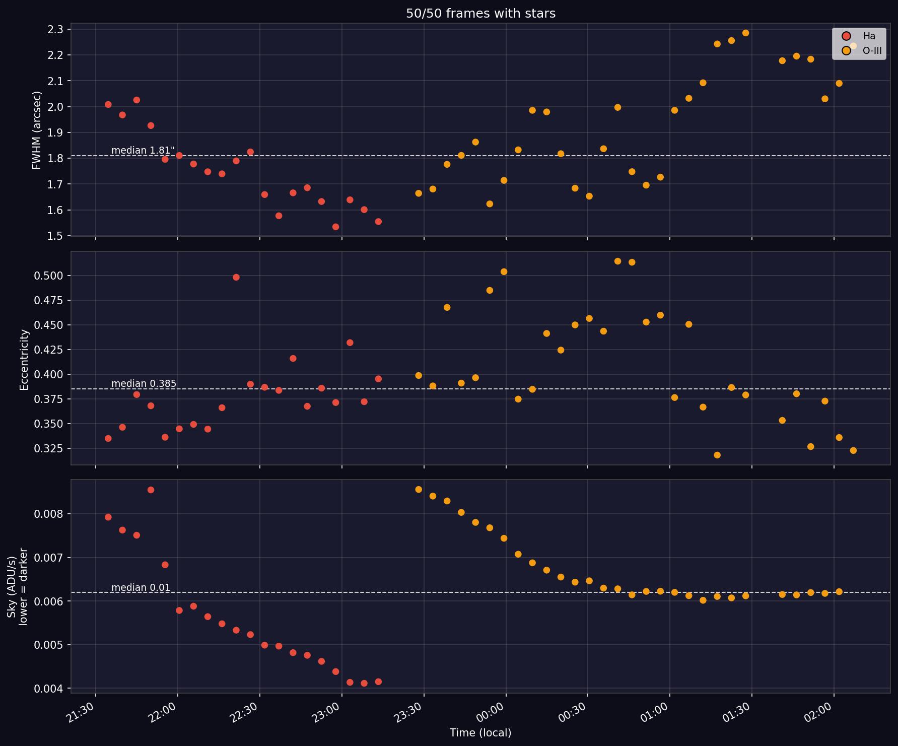
Conditions across the night, measured per frame by the pipeline's own
Moffat fitter:
Frames
Median FWHM
Median eccentricity
Hα
20
1.72″
0.37
O III
30
1.89″
0.39
All
50
1.78″
0.39
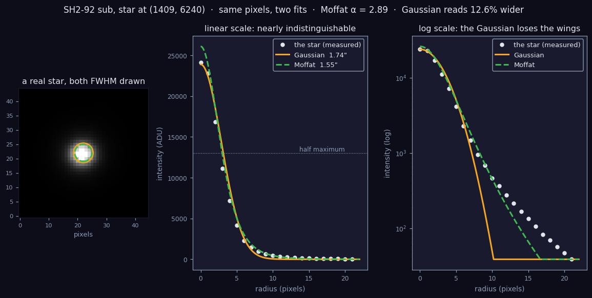
These figures agree with PixInsight's measurements of the same frames to
the second decimal place. That agreement is worth stating because it is
not automatic: the number depends on which profile is fitted, and a
Gaussian fit of the same stars returns a systematically larger width
— the two disagree by 11.5% on this telescope. The pipeline fits a
Moffat profile for width while continuing to take eccentricity and
position angle from a Gaussian, and it is that combination which
reproduces the independent result.
All fifty frames of the night. Seeing drifts from
1.5″ to 2.25″ and the detected star count falls with
it; the step in sky brightness at frame 21 is the filter change
from Hα to O III. The final frame's sky value reads
zero because its background fell below the calibrated pedestal
— a measurement limit rather than a dark sky.
Both stacks contain a thin linear feature. In O III it spans
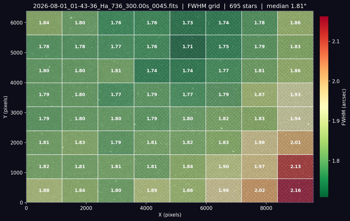
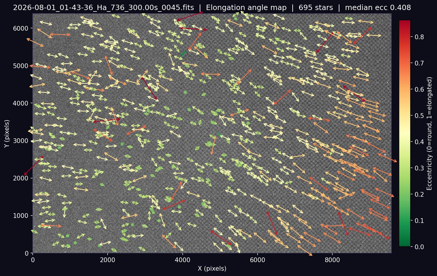
about 55″ — roughly 210 px — at a position angle
of 73°, and is 19–23 px across — about 5″, or roughly
three seeing discs, so it is resolved across its width rather than being
a knife-edge line. A matched-filter search of the Hα stack finds
the same feature at position angle 78°, its ridge centre 14 px
(3.7″) from the O III one. That is closer together than the
strand's own width: the two filters show one feature in one place, as a
sky-fixed feature must, since every filter is registered to a single
shared reference.
The finished composite, with the region containing the
O III strand boxed.High-pass view of the O III stack. The strand lies
between the markers: about 55″ long and
5″ wide.
It is not in the optics or the detector
Anything fixed to the sensor or to the optical train sits at a constant
pixel position. Registration aligns each exposure to the stars,
so such a feature is dragged along the field's drift track and smeared.
The drift on this night was substantial and independently measured —
36.8 px (9.7″) across the Hα sequence and 85.2 px (22.5″) across the O III,
in different directions — so a detector-fixed artefact would have
been smeared by tens of pixels in a direction that does not match the
observed feature.
Four calibration hypotheses were tested by substitution, and all four
were eliminated:
Hypothesis
Test
Result
Flat-field residual
Re-stack with no flats at all
Feature unchanged
Bias or dark residual
Independent reduction, same masters
Feature absent from that reduction
Hot or defective pixels
Defect map from the master dark
Feature unchanged
Filter or window debris
Inspection of the master flats
Not present — but see below
Dust or dirt in the optical path
Stack in detector coordinates instead of sky coordinates
9× weaker — see below
The last of those deserves a correction rather than a tick. Searching the
flats for the feature was proposed as a test and reported as evidence.
It is not evidence: a flat records the detector's response to uniform
illumination, so a feature fixed with respect to the sky cannot appear in
one whether it is real or not. The test had no discriminating power in
either direction. This was pointed out by the observatory's owner and is
recorded here as a correction.
Dust or dirt somewhere in the optical path is the strongest version of
this family of hypotheses, and it makes a testable prediction. Such an
obstruction is fixed to the detector, not the sky. Registration
aligns the stars, so it would be dragged backwards along the field's drift
track and smeared — by 85 px in O III, at a position angle
56° from the strand's own axis, which would broaden a thin feature
across its width by some 71 px. The observed width is 19–23 px.
The direct test is to stack the same exposures both ways and ask which
frame the feature is sharp in:
Combination
Peak
Integrated flux
Registered to the stars
+0.685
+19.27
Detector coordinates, unregistered
+0.174
+2.15
The feature is 3.9× stronger in peak and 9× stronger in
integrated flux when the frames are aligned on the stars. It accumulates
coherently in the sky frame and washes out in the detector frame, which is
the opposite of what any obstruction in the optical path can do. The
residual in the detector frame is not zero only because the drift, 85 px,
is smaller than the feature's own 225 px length, so the smeared copies
partly overlap.
Nor is it a diffraction spike
This hypothesis deserves separate treatment, because it is the one
instrumental explanation that none of the tests above can exclude. The
mount is equatorial, so the field does not rotate: a diffraction spike
keeps a fixed position angle and a fixed offset from its parent star in
every exposure, and therefore in the registered stack. It would survive a
median of thirty frames, and its signal-to-noise would grow with frame
count, exactly as the observed feature does. When this hypothesis was raised, the two filters were
believed to show the feature in different places, which spikes from two
different stars would have explained neatly. That belief later proved
wrong — they are co-located — but the tests below stand on
their own.
It looked promising. Searching the bright stars around the feature found
one at (5750, 5625) whose separation from the strand's infinite axis
is only 34 px over a 528 px baseline — a misalignment of 3.7°,
with the strand lying 416 to 640 px radially outward from it.
Three tests reject it. A spike is brightest at the star and fades
outward, so it cannot begin four hundred pixels away; sampling the profile
along the strand's own bearing from that star shows the opposite of what
is required:
Distance from the star
Mean excess
Expected for a spike
40 – 380 px
−0.0504 ADU
strongest here
380 – 660 px (the strand)
+0.2364 ADU
weaker than the inner region
beyond 660 px
+0.0225 ADU
weaker still
The feature is detached from the star, with nothing in between. Sampling
at 90° intervals for the four-fold pattern a vane spider would produce
gives +0.236, +0.002 and +0.008 ADU in the three usable quadrants; the
fourth ray leaves the frame and returned an edge artefact, so that
quadrant is void rather than negative.
The decisive test is more general: does this telescope produce spikes at
all? Stacking the 63 brightest stars in the field, each normalised to its
own peak, and measuring mean flux by position angle in the 25–100 px
annulus where a spike would be most prominent:
Position angle
Mean normalised flux
15° – 30°
+0.003155 (highest)
median across all twelve bins
+0.001031
60° – 75° (the strand's angle)
+0.000051 (lowest)
There is no coherent spike system, and the strand's own position angle is
the weakest of the twelve bins — the opposite of the
prediction. What mild variation exists peaks near 20° and 140°,
which are 120° apart rather than the 90° a four-vane spider would
impose.
The apparent alignment was therefore coincidence. With eighteen bright
stars in the search box, one falling within 4° of any chosen line is
unremarkable, and it should have been treated as a hypothesis to test
rather than as evidence — the same error recorded at the end of this
note, committed once more.
It is not a satellite, meteor, asteroid or comet
A satellite or meteor crosses the field within a single exposure. The
feature survives a median combination of thirty frames, and a median
discards anything present in fewer than half of them. That excludes both.
Excluding a minor planet or comet requires a different argument, and it is
the argument that settled the question. It arose from a question put by
the observatory's owner: if the object is moving with respect to the
stars, how can stacking make it more prominent?
The arithmetic is decisive. Consider a pixel on the object's track where
it is present in one exposure out of N. The mean of the stack
holds signal S/N at that pixel, while the noise falls as
σ/√N. The resulting ratio is
SNR = (S/N) ÷ (σ/√N) = (S/σ) ÷ √N
a moving object gets √N WORSE as frames are added
whereas a feature present at the same registered pixel in every exposure
gains √N. The two predictions differ by a factor of
N, and they are trivially separable by measurement. Combining
random subsets of the O III exposures gives:
Frames combined
Measured peak SNR
If static (√N)
If moving (1/√N)
2
2.69
2.69
2.69
7
2.94
5.04
1.44
18
3.66
8.08
0.90
29
4.53
10.25
0.71
The measured ratio rises. A moving object would have fallen to 0.71. The
feature is therefore fixed with respect to the stars, and no solar system
body can produce it.
The growth is nonetheless slower than √N. Part of that is
bias in a peak-of-profile statistic at low N, so no exponent
should be read from these four points; but sub-√N growth is
also the expected signature of noise that does not average down, and the
dither on this night was measured at a median step of 0.79″ against a
1.78″ seeing disc — under half a star width — too small to decorrelate fixed pattern between
exposures.
Nor a chip, nor a ghost
A chip or scratch in a mirror or corrector belongs to the same class as
dust: fixed in the optical train, therefore fixed to the detector, and
excluded by the same 9× result. The one variant that escapes that
test is a defect which scatters light from a bright star, since
the resulting artefact would be anchored to the star and, on a mount that
does not rotate the field, would be sky-fixed. Reflecting each of the 25
brightest stars through the optical centre puts the nearest candidate
ghost 704 px — 3.1′ — from the strand. Nothing lands on
it.
The question that should have come first
Every exclusion above treats the feature as though it were singular. None
of them tests that assumption. The test is one matched-filter pass: sweep
the whole stack for lines of the strand's own length and width at every
position angle, and count what comes back.
Quantity
Value
Strand response
8.0σ
Peaks above 4σ in the frame
387
Rank of the strand
20th of 387 — 95th percentile
Population median / 90th / max
6.2σ / 7.5σ / 9.8σ
The strand is not distinctive. Nineteen linear features in the same frame
are stronger, several hundred are comparable, and they lie at every
position angle across the field. It is an unremarkable member of a large
population, and it drew attention only because it happened to fall in a
part of the image that was being examined closely, at a stretch that
showed it well.
That population has an obvious source. This is the Soap Bubble field in
Cygnus, dense with filamentary Hα and O III emission, and a
filter tuned to 55″ lines will respond to real nebular filaments
across the whole frame. Faint nebulosity accounts for every established
property without strain: sky-fixed, identical in both filters, surviving
the median, gaining signal-to-noise with frame count, and untouched by
every calibration substitution. Those are not the signatures of something
exotic. They are what nebulosity does.
The apparent time variation, and what it really was
One measurement resisted every explanation above, and it kept this note
open longer than anything else. Aperture photometry along the feature's
axis, exposure by exposure, is not constant: the first eighteen O III
frames read consistent with zero or negative, the last twelve read
positive at 2.4–7.7σ. Taken at face value the feature appeared
partway through the night, which nothing static explains — and which
sits badly against survival of a thirty-frame median, and against the fact
that the one exposure where the feature is plainly visible by eye falls in
the null group and measures −0.8σ.
Left: the 29-frame stack. Right: one 300-second exposure,
identically calibrated — the feature is present in both, at
the same position relative to the stars. This exposure is the one
the photometry reads as negative.
The obvious hypothesis, raised by the observatory's owner, was pointing
geometry: the target transits 3.7° from the zenith, reaching 86.30°
altitude, and the flux turns positive at 77.07° as the tube tips over
past the meridian. Flexure or a light leak that opens at a particular tube
angle would look exactly like that.
The Hα sequence refutes it, and is able to because it ran
before transit with the target rising, which separates altitude
from time:
Sequence
Altitude below 78°
Altitude above 78°
Hα (rising, pre-transit)
−0.48
+0.61
O III (setting, post-transit)
positive
null / negative
The two filters have opposite altitude dependence. The same
feature cannot brighten with altitude in one and dim with it in the other,
so neither altitude nor tube orientation is responsible.
What the two sequences do share is a flux that climbs monotonically with
time within each block and resets at the filter change. The frame
statistics name the cause: the sky was darkening through each block and
jumping back up at the changeover — 0.00792 to 0.00415 ADU/s
across Hα, a 48% decline, then reset for O III. A
strip-minus-annulus measurement is sensitive to that, and the correlation
is direct:
r = −0.705
measured strand flux against sky brightness, Hα, n = 20
The step at exposure nineteen is the sky background declining, not the
feature appearing. The single piece of evidence that anything unusual was
happening was an artefact of the measurement, and the eye and the
photometry were never really in conflict: the photometry was measuring the
sky.
Errors made in reaching this point
The route to the above included at least six incorrect conclusions,
each stated with more confidence than the evidence supported. They are
recorded because the pattern is more useful than the individual mistakes.
Claim made
What was wrong with it
“Not present in any single exposure”
Rested on a line-detection routine returning nothing. Absence of detection was treated as evidence of absence; the feature is plainly visible in a single frame.
“The mount is not dithering”
A defect in a single-use analysis script. The mount dithers every exposure.
“It is a satellite trail”
Excluded by median survival, which was not tested until much later.
“It is uncorrected hot pixels”
A defect map removed many genuine artefacts and left this feature untouched.
“It is a minor planet at ~20″/hour”
Derived from apparent motion of a 3σ peak between co-added groups — peak-hunting in noise.
“The two filters show it in different places”
Asserted from eyeballing two separately-stretched crops. Measured, the two ridges lie 14 px apart — less than the strand's own width. The claim had already been used as supporting detail when framing later hypotheses.
“It appeared partway through the sequence”
A strip-minus-annulus flux series drifting with the sky background, which fell 48% through each filter block and reset at the changeover (r = −0.705). Presented as the one fact no static explanation could accommodate.
Treating the feature as singular
Never measured how many comparable features the frame held. One matched-filter pass shows 387 above 4σ with the strand 20th. Every exclusion that follows was work spent on a false premise.
“It is settled real structure”
Stated before the photometric series was examined, which contradicts it.
The common failure is straightforward: repeatedly believing three-sigma
structure produced by single-use scripts that had not been validated
against a known answer. A faint feature close to the noise will generate
spurious peaks, spurious trends and spurious apparent motion, and it did
so here more than once. The working rule adopted afterwards is that when a
picture and a number disagree, the number is the one to distrust until the
code that produced it has been checked.
A second observation concerns sequencing. The single most discriminating
test available — how the feature's SNR scales with the number of
frames combined — is also among the cheapest, and it was run last.
Run first, it would have eliminated the satellite, hot-pixel and minor
planet hypotheses in one step and saved the majority of the work.
It should also be recorded that the two decisive contributions came from
the observatory's owner rather than from the analysis. The first was an
independent reduction of the same exposures in PixInsight, using the same
bias and dark frames and no flats, which does not show the feature; that
single control eliminated the entire calibration branch of the
investigation. The second was the question about stacking and moving
objects quoted above, which produced the argument that settled the largest
remaining question. Neither required new data.
Status
Nothing about this feature now requires an unusual explanation. Every
exclusion holds — not the optics, the detector, dust, a chip, the
flats, the bias, the dark, a satellite, a meteor, an asteroid, a comet, a
diffraction spike, nor altitude or tube flexure. What has changed is that
the two facts which made those exclusions seem to point at something have
both dissolved.
The feature is not statistically distinctive: a matched-filter sweep of
its own frame returns 387 comparable linear features above 4σ and
ranks this one twentieth. And it did not vary with time: the apparent step
partway through the sequence was a strip-minus-annulus measurement
tracking a sky background that fell 48% through each filter block and
reset at the changeover.
What remains is an ordinary faint filament in a field dense with them,
recorded on a single night of four hours that was never deep enough to say
more. The recommended observation has not changed and is now the only
thing that would add information: repeat the field on a second night.
Real nebulosity reappears at the same coordinates at the same brightness;
correlated noise does not.
The reservation recorded at the head of this note stands, and the
investigation supports rather than weakens it. Every anomaly here was
eventually located in the analysis — a threshold chosen without a
null distribution, a photometric series contaminated by the sky, a
position claimed from eyeballing two crops — and never in the sky or
in the instrument. That is the finding most worth carrying forward.
A security camera as a scientific instrument
2026-08-10 · ALL-SKY CAMERA · 104° FOV · SOLVED TO 1.5 px · RAIN DETECTOR
Abstract
A $40 Kasa security camera pointed at the zenith turns out to be a
usable instrument, but only after it is plate solved: with the geometry
known, every pixel maps to an altitude and azimuth and limiting magnitude
becomes measurable. Three things came out of using it. Its sensitivity is
strongly radial — star completeness runs 24–39% out to 800 px
from the optical axis and then falls to exactly zero, because the
same star delivers five times less signal at the frame edge; ignoring that
made the completeness table read upside down, finding 43% of
magnitude‑2 stars while magnitude‑6 stars came through. A trail
that looked exactly like a Starlink pass was an insect, settled by
arithmetic rather than opinion: 4.22° in ≤66 ms is ≥64°/s and
low Earth orbit tops out near 1°/s. And seven days of continuous
footage off its own memory card turned it into a rain detector that caught
a six-hour storm the gridded forecast recorded as zero precipitation.
The camera did not change. The geometry did.
The camera is a Kasa KC420WS, a consumer security camera, bolted looking
up. It has no manual exposure, no RTSP, and sends H.264 whatever you ask
it for. On its own it produces a picture with dots in it.
What makes it an instrument is a blind plate solve — the same
method astrometry.net uses, shrunk to fit. Orientation plus focal length
is four unknowns, so two correct correspondences between a detected dot
and a catalogue star pin all four; try every pairing of the brightest
detections against the brightest stars that are up, and keep whichever
hypothesis puts the rest of the catalogue on top of the
rest of the detections. No initial guess needed.
Solved parameter
Value
Focal length
1616.85 px/rad
Projection
equidistant fisheye
Optical axis
4° off zenith (alt 85.9°)
Field of view
104° corner to corner
Plate scale
0.0354°/px (128″/px)
Match residual
1.3–1.5 px
The sanity check that matters is not the residual, it is that the named
stars come out as neighbours. A correct solve names one
contiguous patch of sky. A coincidence names stars scattered across
unrelated constellations.
With that in hand the useful quantity stops being “how many dots did
we count” and becomes limiting magnitude: the
brightness at which the detection rate falls through half. A star count
also drops when a branch grows into the field or more of the frame is
masked. How faint the sky lets you see is a property of the sky.
Sensitivity is a function of radius, and ignoring it inverts the answer
The completeness table — how many catalogue stars of each magnitude
were recovered — came out backwards. Only 43% of magnitude‑2
stars were found, while magnitude‑6 stars, four hundred times
fainter, were coming through. Brightness plainly was not the variable.
Splitting the same measurement by distance from the optical axis explains
it in one step:
Radius from axis (px)
Catalogue stars
Detected
Completeness
0 – 200
31
12
39%
200 – 400
86
24
28%
400 – 600
102
29
28%
600 – 800
117
28
24%
800 – 1000
41
0
0%
1000 – 1200
54
0
0%
1200 – 1500
30
0
0%
Not a gradual falloff — a wall. One hundred and twenty-five
catalogue stars beyond 800 px, none of them recovered. The cause is
off-axis attenuation, and two stars of nearly identical brightness make
it concrete:
Star
Radius (px)
Peak above background
Result
V = 2.20
106
125 ADU
found
V = 2.23
1214
26 ADU
missed
Same star brightness, five times less signal, and the fainter one falls
under the detection threshold. So a bright star that happened to land near
the edge was lost while a faint one near the centre was found, and with
only seven magnitude‑2 stars in the frame, four of them landing
outside 970 px was enough to invert the table.
The fix is to stop counting stars the optics cannot deliver. Those beyond
800 px are dropped from the denominator — the same reasoning already
applied to stars sitting on masked foliage, where counting them would
measure how much of the frame is trees rather than how clear the sky is.
Restricted to the region where the instrument actually works, the table
becomes monotonic:
Magnitude
Before (whole frame)
After (r < 800 px)
found / total
%
found / total
%
2
3 / 7
43%
— too few to bin
3
7 / 11
64%
7 / 8
88%
4
36 / 56
64%
37 / 47
79%
5
31 / 186
17%
32 / 133
24%
6
12 / 206
6%
13 / 144
9%
Limiting magnitude
4.40
4.59
The published frame now draws the boundary it measures inside, so the
picture and the numbers beside it cannot drift apart. It is not a circle:
at 800 px radius the disc overshoots the top and bottom of a
2560 × 1440 frame by 80 px, so what is measured is the
disc intersected with the frame — a disc with both caps sliced flat.
Drawing only the arc left the shape open exactly where it leaves the
picture, which read as though the strips above and below were excluded
when they are counted.
Detections circled, foliage shaded, and the outline of the
region the statistics are measured inside. Detections outside it
— along the left and right edges — are the ones now
excluded.The solve, checked the way that matters: catalogue
positions land on detections, and the named stars come out as
neighbours rather than scattered.
The Starlink pass that was an insect
On 2026-08-08 a long bright trail crossed the frame. It looked exactly
like a satellite pass, and that was the first reading of it. Arithmetic
disagreed.
The camera runs at a measured 15.1 fps, so a single frame integrates for
at most 66 ms. The trail spans 4.22°. That gives a lower bound on
angular rate:
ω ≥ 4.22° / 0.066 s = 64°/sand a satellite in low Earth orbit tops out near 1°/s
Sixty-four times too fast, and that is a lower bound — the
true exposure may be shorter still. Nothing in orbit moves like that.
Something very close to the lens does.
Two independent details agree. The trail is 23 px wide against a stellar
PSF of 2.74 px — 5.8′ against 49″ at this camera's 128″/px — eight times too fat, so badly out of focus, so very
close. And it is beaded: brightness modulated along its length at
a regular pitch, which is a wingbeat strobing against the exposure.
The full frame. At a glance, a textbook satellite pass.Zoomed: the beading. Regular modulation along the track is
a wingbeat, not a spacecraft.
The general lesson is that the whole chain rested on one measured number,
the frame rate. Because the insect identification was later confirmed
independently, it also became indirect evidence that 15 fps holds in full
darkness — the frame rate had only ever been measured near dawn.
From counting stars to detecting rain
The camera records continuously to its own memory card, which turned out
to hold seven and a half days of one-minute video segments — roughly
11,000 minutes, 2560 × 1440 at 15 fps. Rain history
that would have taken a season to collect deliberately already existed.
Rain is not subtle on this camera, because its infrared illuminator lights
raindrops a few centimetres from the lens. What arrives is not a picture
of weather at a distance; it is near-field, wildly defocused streaks
filling the frame.
Heavy rain, 2026-08-06 03:45. The gridded forecast recorded
zero precipitation for this hour.The same camera on a clear night. Mean level 16.7 ADU
against 89 in rain — but that difference is the illuminator,
not the weather.
Absolute brightness is the wrong signal precisely because of that
illuminator, and because auto-exposure renormalises every frame. The
measurement has to be scale-invariant. What works is motion
between adjacent video frames: the fraction of pixels whose value
changes by more than 12 ADU from one frame to the next, 66 ms apart.
Sidereal drift over 66 ms is 0.0078 px, so stars are static to a
hundredth of a pixel. Anything that moves is not a star, with a hundredfold
margin. The metric is computed only inside the 800 px region established
above, which excludes the tree line entirely, so wind cannot fake it.
Twenty-four consecutive frames, 1.6 seconds. This is what
the detector is measuring — not brightness, but how much of
the frame changes between one frame and the next.23.4 mm of rain falling, in daylight. No illuminator, so no
lit drops, and the detector reads 7%. This is its hard limit.
The separation is not marginal:
Condition
Pixels changing between frames
Clear night
0.1 – 1.1%
Rain
16 – 100%
Daylight rain
3 – 7% — not detected
It found a storm the forecast did not have
Scanning the whole card at 15-minute sampling and scoring every hour
against Open-Meteo's hourly precipitation gives the honest test. Night
rain is caught reliably, and the hour-by-hour profile tracks the storm
ending: 85% → 100% → 16% → 39% → 19% → 1.8%
across the 22:00 hour on 2026-08-07.
The interesting result is a disagreement. For six consecutive hours on
2026-08-06, midnight to 05:00, the detector read 40–69% while the
gridded model reported zero precipitation. The frames
settle it — that is the heavy rain pictured above. The observatory
sits on a hilltop, and this is the case where a local instrument beats a
model interpolated from distant stations.
That is also the argument for wiring it to the roof. A forecast that
misses the storm entirely cannot protect anything.
How much warning does it give?
Rain onset is a ramp, not a step, which means a lower threshold buys
warning. Measured at two-minute cadence through two storms, using three
consecutive samples over threshold so that isolated spikes do not fire:
Storm
>1%
>3%
>10%
>30%
1% → 10%
2026-08-06
23:44
23:56
00:10
00:36
26 min
2026-08-07
19:52
20:20
20:30
20:32
38 min
Two caveats keep this honest. The 08-07 storm arrived at dusk, and its 1%
crossing happened while the camera was still in daylight mode where the
detector does not work; the trustworthy figure there is the 3% crossing at
20:20 once the illuminator came on, which is 10 minutes,
not 38. So useful warning is 25–40 minutes for a storm arriving in
full darkness, and close to none for one arriving at sunset.
And escalation is not gradual. Going from 10% to 30% took 26 minutes on
one storm and two minutes on the other. The early ramp is
a reliable warning; what happens after the threshold is not. A 10%
crossing should be read as “already raining hard”, never as
“getting worse slowly”.
Two other signals were tested as precursors and both failed. Star count
collapses when cloud arrives — on 08-06 stars went from 13 to
near zero at 21:40 — but rain did not start for another two and a
quarter hours. Cloud precedes rain by far too much, and too unreliably, to
trigger on. Frame level was flat across the run-up. The working model is
single-signal: motion, with persistence.
Where the ceiling is
Two limits are structural, both because this is a consumer camera, and
neither is worth planning around as fixable.
No manual exposure. Auto-exposure renormalises every
frame, so absolute brightness carries no information and every metric must
be scale-invariant. This is exactly why limiting magnitude works where
mean luminance does not, and why the rain detector counts changed pixels
rather than measuring how bright the frame got.
H.264 everywhere. Stacking twelve frames gave a 1.04×
noise reduction against an ideal of 3.46×, because only 1.6% of
pixels genuinely change between adjacent frames — the encoder's skip
blocks reproduce the previous frame bit-identically and hand back copies of
noise that was already discarded. Photometry on such frames is suspect, and
V ≈ 4.4 is about where the instrument stops.
There is also a false-positive mode worth naming: twilight. At sun
altitude −9.4° the frame level drifted 8.4 ADU within a
single burst as dawn came up and auto-exposure hunted, and the whole
frame registered as moving. Gating on sun altitude below −10°
— the same definition of night the scheduler already uses —
removes it.
Postscript: the camera moved, and the calibration went with it
Reading the memory card meant taking the camera down. It went back
pointing somewhere slightly different, and that single physical act
invalidated everything geometric built on top of it: the compass headings
drawn on the published frame, the outline of the region the star
statistics are measured inside, and limiting magnitude, which cannot be
computed without knowing which catalogue stars should have been in view.
The pipeline notices — it verifies the stored solution against every
capture and reports when it stops fitting — but noticing is not
fixing.
The recovery had been a manual procedure, which is the wrong shape for
something that will happen again. It is now a single web-chat command
that captures a frame, blind-solves it, and saves the result only if it
verifies at least as well as the solution it would replace, keeping the
old file alongside. It refuses to run on anything it cannot solve
honestly: daylight, too few stars, or a frame the negative-image control
calls untrustworthy, which is what cloud and rain look like and would
have it matching noise. It reports how far the axis moved and posts the
re-annotated frame so the new compass headings can be checked by eye.
The general lesson is worth separating from the incident. A solved
instrument carries a calibration that a physical act can invalidate
silently, and the cost of that calibration being wrong is not an error
message but a set of plausible-looking numbers that are no longer about
the sky. The recovery path deserves to be one command, available at the
moment conditions allow it, rather than a procedure to be remembered.
What it is good for next: an artificial horizon that maintains itself
This observatory does not plan against the geometric horizon. It plans
against the tree line, which reaches 83° altitude in the worst
direction and has a median of 49° — the site is heavily
obstructed, and the difference between the two horizons is most of the
observable sky. That tree line currently lives in a hand-measured file of
thirty-three azimuth and altitude pairs.
A hand-measured horizon has two problems. It is coarse, at roughly one
sample every eleven degrees of azimuth. And it is a snapshot: trees grow,
limbs come down, trees are removed, and the file does not change unless
somebody remembers to change it. An observatory that plans four hours of
imaging against a horizon measured years ago will quietly lose frames to
branches that were not there at the time.
The all-sky camera already produces the raw material for a better one. It
segments foliage in every capture — on level rather than texture,
because at night exposure the trees are too dim to be rough but sit
10–22 ADU above a ~2 ADU sky — and that mask covers
15–33% of the frame depending on conditions. With the plate solve,
every masked pixel has an altitude and azimuth. The mask is a
horizon profile, already measured, several hundred times a night, in sky
coordinates.
Accumulating those masks over many clear nights and taking a high
percentile per azimuth bin would give a dense profile that is robust to a
passing cloud or a bird, updates itself as the vegetation changes, and
needs no ladder.
Two limits apply to the all-sky camera doing this job, and together they
argue for a different camera. The first is parallax: it sits beside the
telescope rather than on it, and an offset d subtends roughly
arctan(d/D) at a tree line distance D —
about 4° for a two-metre offset and trees thirty metres away. Small,
but the same order as the improvement being sought. The second is
coverage: its optical axis sits 4° off zenith and its field reaches
about 52° from that axis, so it cannot see below roughly 34°
altitude, while the existing profile runs down to 25°.
The intended solution is the webcam already mounted on the CDK tube
itself — the same camera the observatory uses for its parked-scope
and roof-open safety checks. Being on the tube, it is effectively
co-located with the aperture, so the parallax term vanishes: the horizon
it sees is the horizon the telescope sees, which is the quantity
the scheduler actually needs. It also looks along the optical axis, so it
reaches the low bearings the all-sky camera cannot.
This changes the method rather than the principle. A tube-mounted camera
points wherever the telescope points, so instead of one all-sky mask per
capture it gives a narrow view of a single bearing at a time, and the
profile has to be assembled from many pointings — accumulated
opportunistically as the mount works through a night, or swept
deliberately in azimuth once. The foliage segmentation and the
pixel-to-sky mapping are the same problem either way; only the sampling
strategy differs.
None of this needed better hardware. It needed knowing where the camera
was pointing, which region of it works, and which of its numbers mean
anything.
What shape is a star?
2026-08-07 · POINT SPREAD FUNCTION · GAUSSIAN vs MOFFAT · 11.5% APART
Abstract
A star is a point source, yet it lands on the sensor as a blob several
pixels across. The shape of that blob — the point spread function
— is what every measurement of “seeing” actually
measures, and the number depends on which function you fit to it. This
derives the FWHM from first principles for both the Gaussian and the
Moffat, shows where the constant 2.3548 in the code comes from, and
explains why the two disagree by a systematic 11.5% on this telescope:
1.76″ against 1.56″ on the same 118 stars. The Moffat wins
because atmospheric wings follow a power law that a Gaussian cannot
represent, so the Gaussian widens its core to compensate. It is also why
PixInsight has always reported lower seeing than this pipeline did.
The question
A star is, for any telescope ever built, a perfect point —
unresolvably far away. Yet it arrives on the sensor as a smear several
pixels wide, and how wide it is happens to be the most-quoted number in
amateur astronomy. That smear is the point spread
function: what the atmosphere and the optics do to a point of
light on its way to a pixel.
Reporting its width means choosing a function to fit, and the choice is
not cosmetic. Fit two different functions to the same star and you get
two different answers, both defensible, differing here by 11.5%. That is
larger than most of the effects an observatory is trying to detect.
The Gaussian, and where 2.3548 comes from
The obvious first choice is a Gaussian, on the reasoning that many
independent random perturbations tend toward one:
I(r) = A exp( −r² / 2σ² )
A = peak intensity · r = distance from centre · σ = width parameter
σ means nothing to an observer at the eyepiece, so width is quoted
as the full width at half maximum: how wide the profile
is at half its peak brightness. Deriving it takes three lines. Set the
intensity to half the peak and solve for r:
That r is the half width, so the full width is twice it:
FWHM = 2σ √(2 ln 2) = 2.3548 σ
There is the magic constant that appears unexplained in almost every
piece of astronomy software, this pipeline included. It is not a fudge
factor or a calibration — it is 2√(2 ln 2), and it follows
from the definition of half maximum and nothing else. For an elliptical
star the two axes combine as a geometric mean,
FWHM = 2.3548 √(σxσy),
which is the width of the circular Gaussian covering the same area.
The Moffat
The Gaussian has a problem that only appears far from the centre.
Moffat’s 1969 profile replaces the exponential with a power law:
I(r) = A [ 1 + (r/γ)² ]−αγ sets the core width · α controls how fast the wings fall away
Two functions, two derivations, one definition of width. And the
Gaussian is not a rival so much as a limiting case: as
α → ∞ with γ = σ√(2α), the
Moffat becomes exactly the Gaussian, because
(1 + x/α)−α → e−x.
The Gaussian is the Moffat with infinitely steep wings —
which is precisely the assumption that fails.
Why they disagree: the wings
Far from the centre the two behave completely differently. The Gaussian
falls as e−r², faster than any power law and
effectively zero within a few σ. The Moffat falls as
r−2α — a power law, which keeps a little
flux at large radii indefinitely.
Atmospheric turbulence produces power-law wings, so a real star has more
light far from its centre than a Gaussian permits — visible in the
right-hand panel below, where the Gaussian hits zero while the star is
still clearly shining. The fitting routine
has to reconcile that somehow, and it does so by widening the
core: a broader Gaussian captures more of the wing flux at the
cost of misrepresenting the middle. The reported FWHM comes out too
large, systematically, for every star, on every frame.
A Moffat has no such conflict. Its α absorbs the wings while
γ describes the core, so the two are fitted independently instead
of traded against one another. For Kolmogorov turbulence
α ≈ 4.8; smaller values mean heavier wings.
One real star from an SH2-92 sub-exposure, at pixel (1409, 6240),
with both profiles fitted to the same pixels. Left:
the star, with each fit’s FWHM drawn as a circle — the
Gaussian in orange is visibly the wider of the two.
Centre: the measured radial profile on a linear
scale, where the two fits are almost impossible to tell apart, which
is exactly why this discrepancy went unnoticed for so long.
Right: the same data on a log scale, where the
disagreement is obvious. The Gaussian collapses to nothing beyond
about 10 pixels while the star keeps emitting light out to 20 and
beyond. Note that the measured points sit above even the
Moffat in the far wings: the real profile is heavier still, so the
Moffat is a better description rather than a perfect one.
Click for full size.
What it measures here
Both functions fitted to the same 118 bright stars in one SH2-92
sub-exposure, on identical pixels:
Profile
FWHM (px)
FWHM (arcsec)
Gaussian
6.77
1.76″
Moffat
6.00
1.56″
The Moffat reads 11.5% smaller, in the direction the
theory predicts. This also settles a long-standing niggle: PixInsight has
consistently reported better seeing than this pipeline, and the reason is
simply that PixInsight fits a Moffat. Neither was wrong. They were
measuring the widths of two different functions and both calling the
answer FWHM.
What changed, and what deliberately did not
The pipeline now fits both profiles to every star. Width comes
from the Moffat; shape — eccentricity and major-axis angle —
still comes from the Gaussian. That is not indecision. The standard
Moffat implementation is circularly symmetric: γ and α and
nothing else, so it cannot express elongation at all. Swapping wholesale
would have silently deleted the very numbers the optics-trend metrics
use to detect tilt, coma and collimation drift. Two fits, each asked only
what it can answer.
Historical measurements were tagged, not converted. It
is tempting to scale the old Gaussian numbers by 11.5% and keep one
continuous series, but that figure is not a constant — it depends
on α, which varies with the seeing on the night. Scaling would
manufacture a precision that was never measured. Records now carry the
model that produced them, the trend code refuses to mix the two
families, and the single night of existing baseline was recomputed from
its original frames rather than adjusted. The frames are the archive;
every derived number is only a cache.
A search that finds nothing looks exactly like a search that works
2026-08-05 · INJECTION TESTING · 3 BUGS IN THE PIPELINE · 4 IN THE TEST
Abstract
A supernova search that had reported nothing for weeks turned out to be incapable of detecting a supernova — and no amount of reading its output would have revealed it, because a working detector and a blind one both print “no candidates”. Injecting fake sources of known brightness into real frames exposed three pipeline bugs in a single run: a shape cut that rejected 85% of genuine point sources, a mask that deleted the brightest transients by construction, and catalogue identification that had been dead for 67 commits. It also exposed four bugs in the test itself. The closing argument is why the standing assertion is monotonicity rather than a pinned number: a conventional regression test would have recorded the broken behaviour as correct and failed the repair.
The question
The supernova search had been running for weeks and had found
nothing. That is the correct result — one amateur telescope
revisiting a couple of dozen galaxies should discover approximately
none — and the note describing it said so with some confidence.
But it also carried a caveat that turned out to be the only
interesting sentence in it: a non-detection is worth exactly what
its sensitivity is. "Nothing found" is a statement about the sky
only if you know how bright a real event would have had to be to
survive the filtering. Otherwise it is a statement about the
software. And the two are indistinguishable from the output, because
a detector that is working perfectly and a detector that is
completely blind both print "no candidates".
That is an uncomfortable position for every cut in the pipeline. Each
one was added because it removed false positives, and each one
demonstrably did. Nothing in a normal run reveals whether it also
removed the real thing.
The method: stop waiting for a supernova
A supernova cannot be summoned on demand, so the answer is to inject
fake ones. Take the real frames from a real night, paint in synthetic
point sources of known position and known brightness, run the entire
unmodified pipeline, and count how many come back. The result is a
completeness curve: recovery fraction against brightness. It
is standard practice in professional surveys for exactly this reason,
and the script to do it had been sitting in the repository, unrun.
Two words are doing a lot of work here, and neither means quite
what it sounds like. The template is a deep image
of the same patch of sky, built by stacking every previous
night. The science image is the most recent
night's stack. Both are ordinary exposures of the target and differ
only in when — neither has anything to do with
calibration frames, the bias, dark and flat exposures that remove
the instrument's own signature. Subtract "before" from "now", and
what remains is what changed.
Two details then decide whether the exercise means anything. The
injections go into the real registered science frames, so they carry
the night's actual noise, sky and galaxy underneath — only the
source is synthetic. And they are injected into the science image
only, never the template, so they look precisely like something that
appeared since the last visit.
The first run answered the question immediately
It produced this, on NGC 5907:
Injected flux (ADU)
Recovered
100
0 / 3
200
0 / 3
400
2 / 3
800
0 / 3
1600
0 / 3
3200
0 / 3
6400
0 / 3
This is not a detection limit. It is impossible. A source
sixteen times brighter cannot be harder to find than one at 400 ADU,
and no amount of noise produces that shape. The curve is not a
measurement of the sky; it is a bug report about the detector, and it
took one run to get it.
Three bugs, and none of them were visible in normal output
The shape window was tuned backwards. A supernova is
a point source, so the search kept only compact round residuals
— semi-major axis between 0.6 and 1.3 pixels, said to match
"measured stellar a ≈ 0.7". That figure does not
describe this telescope. Measured on the stack: real stars have median
a = 2.51 (FWHM 5.6 px), and residuals in the difference
image 2.83. The window was admitting 15% of genuine point
sources and rejecting the rest as "extended" — it was
selecting for the sub-pixel artifacts it existed to exclude.
Where the 0.7 figure came from is still unknown. A hot-pixel origin
was proposed here and then withdrawn: the frame-statistics code was
the obvious suspect, but tested against normal frames it measures
stars correctly, so it did not produce that number.
Widening it to the measured stellar spread raised recovery from 2/21
to 8/21 and lowered false positives from 5 to 3. That is the
detail worth pausing on: this was never a trade between sensitivity
and purity. The cut was simply worse on both axes, and had been for
as long as it existed.
Bright transients masked themselves out. Saturated
stars subtract badly, so the pipeline masked the top 0.1% of pixels
and rejected anything landing inside. It built that mask from the
science image — and a bright supernova is, by
definition, among the brightest pixels of the science image. Every
injection at or above 3200 ADU was being discarded as a saturated
star. The brighter the event, the more certain its rejection.
Saturated stars are in the template too, so building the mask from
the template alone loses nothing: false positives stayed at 3 while
recovery went from 8/21 to 14/21.
Identification had been dead for 67 commits. A
refactor on 17 July changed a shared function to take a solved
astrometric position instead of a file path. The transient search was
never updated, so every call raised a type error — into a
try/except that logged it with the same bland message
used for a failed network lookup. For three weeks the search produced
no coordinates, no catalogue cross-match and no object names. And
because the alert rule is "notify if bright and not a known
star", the clause that suppresses alerts for catalogued variables
could never be true: every bright variable was paging a phone as a
possible discovery.
After all three, on the same field and filter:
Injected flux (ADU)
Before
After
100
0 / 3
0 / 3
200
0 / 3
0 / 3
400
2 / 3
3 / 3
800
0 / 3
3 / 3
1600
0 / 3
3 / 3
3200
0 / 3
3 / 3
6400
0 / 3
3 / 3
Monotonic, against one false positive on the un-injected difference.
The honest summary of the previous weeks is that the search could not
have found a supernova: anything with a normal stellar profile was
cut as extended, and anything bright was masked as a saturated star.
The narrow band where those two failures did not overlap was roughly
400–800 ADU, and even there recovery was about 2 in 21.
The discovery underneath the bugs
Fixing the shape window exposed something more awkward than the bug.
The injected sources all have an identical profile, so their measured
size should be identical too. It is not:
Injected flux
400
800
1600
3200
6400
Measured semi-major axis
1.06
1.90
2.29
2.47
2.66
Same physical width, two and a half times the measured size. The
detector's size estimate is a second moment over pixels above the
detection threshold, and a brighter source lifts more of its wings
above that threshold. So size is not independent of
brightness, and any fixed size window is a brightness cut in
disguise. The window in place now is bounded by measurement
rather than by a mis-remembered number, which is an improvement, but
the right answer is a shape test that compares each candidate against
the frame's own stars at matched brightness. That is a redesign, not
a tuning change, and it has not been done.
Turning the same question on the exoplanet search
If a detector can be structurally blind while looking healthy, the
transit search deserved the same treatment — more so, because it
carries the more prominent claim. HAT-P-32b was found and ranked
first, which reads as evidence the search works.
The transit version injects the opposite sign: a box-shaped dip of
known depth, multiplied into a real star's raw flux before every
normalisation step, so a synthetic transit faces everything a real one
does. It has not yet produced a trustworthy depth floor, for reasons
given below, but it produced one number immediately that needs no
calibration at all: of 1055 stars detected in the field, 490
are searched. The edge margin, validity threshold and
saturation cut discard 54% of the field before any transit scoring
happens. A planet transiting a star in that other half is invisible at
any depth. Whether those cuts are right is a separate question; that
they halve the survey was not written down anywhere.
Four bugs in the test itself
The instrument measuring the instrument needs the same scepticism, and
it earned it. Every one of these produced a confident, wrong result
before being caught:
Mistake
Symptom
Injections placed on stars the search never examines
0% recovery at every depth, including 4%
All injections given one shared epoch
correlated dip, correctly removed by the detrending it was supposed to survive
Epoch rounded to five decimals when recorded
depth silently under-delivered by 10%
Targets chosen by brightness, not photometric quality
same 4% dip at SNR 12.4 on one star and 1.8 on another
The last one is why no transit depth floor is quoted here. Brightness
is not precision, and with targets spanning that range the curve
describes the noise of arbitrarily chosen stars rather than the
sensitivity of the search. Selecting targets by lowest scatter is the
fix and is not yet done.
The assertion that caught all of it
Every failure above — three in the pipeline, four in the test
— announced itself the same way: recovery that did not increase
with signal strength. That is now asserted in both tests, and it is
worth being precise about what is asserted, because the obvious choice
is wrong.
A conventional regression test pins current behaviour and fails when
it changes. One written against the supernova search the day before
would have recorded "recovery = 2/21" as correct, and then failed the
moment the shape window was fixed — reporting the repair as a
regression and defending the bug. Completeness is supposed to
improve, so pinning it is worse than not testing at all.
What cannot legitimately change is the shape. A stronger signal must
not be recovered less often than a weaker one. That is physics rather
than tuning, so it survives any amount of genuine improvement while
still catching every failure listed here. The tests now enforce it and
exit non-zero when it breaks, which makes them a standing check rather
than a thing that was run once.
Writing the check produced two more bugs, in the check. A real failure
— the deepest transit recovered zero times while a shallower one
was found — passed, because the drop sat exactly on the
tolerance. And a legitimate one-sample wobble failed, because
2/3 < 1.0 - 1/3 is true in floating-point arithmetic.
Both are fixed: comparisons are integer counts, and total failure at
the strongest signal is checked with no tolerance at all, since the
easiest case failing outright is never noise.
What this still does not answer
No limiting magnitude yet, and the reason is worse than
"not done". Two identical runs of the fixed supernova
search put the 50%-recovery floor at 400 ADU and then at 800 ADU,
and produced 662 and 892 raw residuals from the same input frames.
A factor of two in the sensitivity, run to run, with nothing
changed. Until that is understood there is no stable number to
convert into a magnitude, and quoting one would be inventing
precision. The monotonicity invariant held in both runs, which is
the argument for asserting shape rather than a remembered value.
The result that survives all of this is not a detection limit. It is
that the pipeline spent weeks reporting a clean, plausible, entirely
meaningless negative, and that no amount of reading its output would
have revealed it. The only thing that did was giving it a question
whose answer was already known.
Looking for something that was not there last night
2026-08-05 · DIFFERENCE IMAGING · RUNS UNATTENDED ON THE GPU BOX · SUPERNOVAE FOUND: 0
Abstract
How the transient command hunts supernovae by subtracting a deep template built from every previous night from the most recent night’s stack. Most of what survives a subtraction is not astronomy, so the bulk of this is about telling a real point source from misregistration dipoles, hot pixels and galaxy structure — and then from the far likelier explanation, a catalogued variable star. Runs unattended on a separate GPU machine after the night’s frames are copied across, and raises a Pushover alert above a threshold. No supernovae found, which is the expected result.
The question
A galaxy photographed twice looks the same both times. That is the
whole difficulty. Somewhere in a spiral arm a star may have exploded
since the last visit, and it will be one dot among several thousand
dots, sitting on top of a bright, structured, wildly uneven
background. Blinking two images by eye is how this was done for
decades and it does not scale past a handful of fields.
The transient command — diff is the
same thing — asks the question mechanically instead. It gathers
every sub ever taken of a target in one filter, splits them by night,
builds a deep template from every night except the most
recent, treats the most recent night as the science image,
and subtracts one from the other. What survives the subtraction is,
in principle, what changed.
Why subtracting two images is harder than it sounds
The two images are never the same image. The telescope was pointed
slightly differently, the seeing was better on one night than the
other, and the sky was brighter or darker. Subtract them naively and
every star in the field leaves a residual, because a star that is
1.9″ wide on one night and 2.4″ on another does not
cancel. So before subtracting, both are registered onto a common
pixel grid, the sharper one is deliberately blurred to match the
softer one, and the background and scale are matched robustly. Only
then is the difference meaningful.
Even done properly, most of what survives is not astronomy. This is
the part worth being honest about, because the first real run said so
loudly: on NGC 5907 the search returned five candidates at
signal-to-noise between 1200 and 7800, numbers that would be
extraordinary if any of them were real. All five were artifacts.
The thousand-sigma figures were themselves the clue. Significance was
being measured against the noise of the whole frame, and NGC 5907 is
an edge-on galaxy with a bright core — a large, genuinely bright
structure that dragged the global noise estimate down and made every
residual look impossibly significant against it. Noise is now measured
in an annulus around each candidate, so a residual is judged against
its own neighbourhood rather than against an average dominated by
somewhere else in the picture.
What a supernova has to look like
The rest of the tuning is a set of statements about what a real
transient is, each one aimed at a specific thing that was being
mistaken for one:
Test
Cut
What it rejects
Local significance
≥ 5σ vs annulus
noise, and the bright-core inflation above
Source size
semi-major 0.6–1.3 px
hot pixels below, galaxy knots above
Roundness
elongation ≤ 1.4
trails, edges, spiral-arm structure
Negative lobe nearby
≥ 4σ within a scaled radius
subtraction dipoles from misregistration
Bright-source mask
inside the mask
saturated-star residuals
Newness
template flux ≤ 50% of science
stars that were always there
Gaia cross-match
within 2″
catalogued stars — down-ranked, not deleted
The size window is the one that carries the most weight, and it is
measured rather than chosen. This telescope undersamples: real stars
on these frames come out with a semi-major axis of about 0.7 pixels
and an elongation near 1.0. A supernova is a point source, so it must
look exactly like a star and nothing else. Anything meaningfully
larger is galaxy structure; anything smaller is a single hot pixel or
a cosmic ray. Two cuts, one measurement.
The dipole test deserves a mention because it catches the failure that
looks most like a discovery. If registration is off by a fraction of a
pixel, subtracting a star leaves a bright crescent beside a dark one.
The bright half alone is a compact, round, significant, apparently new
source. Looking for the matching dark lobe nearby is what tells them
apart, and the search radius scales with the source, because the wide
dipoles thrown off by an edge-on galaxy's structure put their negative
half further out than a fixed radius would ever reach.
Then the harder question: what is it?
Finding a new point of light is the easy half. The overwhelmingly
likely explanation for a star-like object that brightened is a
variable star in our own galaxy, not a supernova in a distant
one. So surviving candidates are cross-matched against Gaia, and
anything within 2″ of a catalogued point source is heavily
down-ranked — down-ranked rather than deleted, since a supernova
can sit close to a foreground star by chance and silently discarding
it would be the one unrecoverable mistake. A SIMBAD lookup then puts a
human-readable name and object type on whatever matched, which usually
ends the question immediately.
On NGC 5907 the tuned search returned one marginal candidate instead of
five spectacular ones. Identification resolved it to a magnitude-17
Gaia star 0.24″ away. Not a supernova — but the pipeline
said so itself, which is the outcome that matters.
Where it runs
None of this happens while the telescope is working. Once the night's
lights and calibration frames are complete they are copied across to a
separate NVIDIA machine, and the search runs there unattended on
what arrived. The observatory PC stays a real-time controller with a
roof and a mount to worry about; the GPU box does the arithmetic in
the morning, when being slow costs nothing.
If a candidate clears signal-to-noise 8 and is not already a
catalogued star, a Pushover notification goes out with the position
and the triptych image — template, science, difference, side by
side, which is the view that lets a human dismiss most things in about
two seconds. Everything else is written to a JSON file to be looked at
whenever. An alert that fires for every marginal blob would be
switched off within a week, so the bar to interrupt somebody is
deliberately higher than the bar to record a candidate.
Result
No supernovae. This is the correct and expected result: a single
amateur telescope revisiting a couple of dozen galaxies should
discover approximately none, and a pipeline that had found one in its
first weeks would be more likely broken than lucky. What the work
bought is a search that produces one honest marginal candidate instead
of five confident wrong ones.
A non-detection is only worth what its sensitivity is.
"Nothing found" means nothing at all without knowing how bright a
real transient would have had to be to survive those cuts —
a set of filters tuned until the false positives went away can
always be tuned until the true positives go too. There is an
acceptance test that answers this by injecting fake sources of
known brightness into the science frames and measuring what
fraction come back, which is the only way to get the number
without waiting for a real supernova. It has since been
run, and it found that this search could not have detected a
supernova at all. What happened next is its own note:
a search that finds
nothing looks exactly like a search that works. The cuts
described above are the corrected ones; the note explains what
they were, and why the difference was invisible.
Learning to denoise without ever seeing a clean image
2026-08-04 · NOISE2NOISE · U-NET, ~7M PARAMS · STATUS: TRAINING, NOT IN THE PIPELINE
Abstract
Every sub-exposure is mostly noise, and the obvious fix — train a network to map noisy images to clean ones — is unavailable, because no clean image of a galaxy exists anywhere to train against. Noise2Noise removes that requirement: map one noisy frame to another noisy frame of the same scene and you converge on the same model, because the noise carries no learnable information. An observatory turns out to be close to the ideal case for it. Covers what was built, four ways it goes wrong — dithering teaches the network that stars are noise — and why nothing consumes the output yet.
The question
Every sub-exposure this observatory takes is mostly noise. A 300-second
frame of a faint nebula carries read noise from the sensor and shot noise
from the photons themselves, and the target is often fainter than either.
The classical answer is to take a lot of frames and average them, which is
what the stacker does, and it works: noise falls as the square root of the
frame count. The question is whether a neural network can do better than
the square root — whether it can recognise what sensor noise looks
like on this camera and remove it, rather than merely averaging it away.
The obvious way to train such a network is supervised learning: show it a
noisy image, show it the clean truth, and penalise the difference. That
approach is unavailable here, and not for want of effort. There is no clean
image of a galaxy. Nobody has one. No exposure is long enough, no sensor
cold enough; the ground truth does not exist anywhere in the universe to be
collected. Every supervised denoiser needs a target that astronomy
fundamentally cannot supply.
The trick, which is the interesting part
Noise2Noise removes the requirement. The insight is that you can train the
network to map one noisy frame to another noisy frame of the same
scene, and get the same model you would have got from clean targets.
The reason is a property of the loss function rather than of the network.
Training minimises the expected error against the target, and the predictor
that minimises squared error against a random target is that target's
mean. If the noise is zero-mean and drawn independently for each
frame, then the mean of the noisy target is exactly the clean signal. So
the network is being asked to predict something whose expected value is the
truth. It cannot predict the specific noise in any particular target frame
— that noise is independent of its input, and therefore carries no
learnable information — so the best it can do is output the underlying
signal. The noise averages out inside the loss instead of inside the stack.
Put another way: the network learns whatever the two frames have in common
and discards whatever differs between them. Point it at two views of the
same sky and what they have in common is the sky.
An observatory turns out to be close to the ideal case for this. The method
needs many independent noisy observations of an unchanging scene, which is
an awkward thing to arrange for photographs of the physical world —
and it is precisely what a telescope produces by accident. Three hundred
frames of the same nebula on the same filter, each with its own independent
draw of read and shot noise, are the by-product of a single ordinary night.
The training pairs cost nothing; they had already been collected and stacked
and archived before the idea came up.
What is built
A four-level U-Net of about seven million parameters, single channel in and
out, trained per filter and per exposure time — the noise character of
a 90-second red frame is not that of a 300-second H-alpha frame, so they get
separate models. Training draws random 256-pixel patch pairs from two
different frames, 2000 pairs an epoch for 130 epochs, with the same random
flip and rotation applied to both members of a pair so they stay aligned.
Inference runs in 512-pixel tiles with 64 pixels of overlap, because the
QHY600 sensor is 9576×6388 and will not fit in video memory whole.
272aa6e
Four ways to get it wrong
Every one of these was found the hard way, and each is a variation on the
same theme: the method erases whatever differs between the two frames, so
any difference you failed to think about is a thing it will destroy.
Dithering deletes the stars. The telescope deliberately
shifts the pointing a few pixels between exposures, so that sensor defects
do not land in the same place every frame. This is good practice for
stacking and fatal for Noise2Noise. If the scene has moved between input and
target, then the stars are among the things that differ between the two
frames — and the network duly concludes that stars are noise and
learns to suppress them. Frames now get registered to a common reference by
matching star centroids before any training happens. Registration is not a
refinement here; it is a correctness requirement, and the failure it
prevents looks like a beautifully smooth image with the astronomy removed.
8c1afd2,
67a1c9a
Pairs must be the same scene. Nothing in the loss function
knows what a scene is. Pair a frame of M13 with a frame of NGC 7331 and the
maths still runs — it just now describes a network learning to predict
the average of all sky, since that is what those two frames have in common.
Pairs are restricted to within one target, which then made the definition of
"one target" load-bearing: an early version grouped frames by directory
depth and grouped by night instead, silently splitting one object
across sessions.
737e79e
Squared error is the wrong loss for a starfield. The
argument above is cleanest for squared error, whose optimum is the mean.
But a starfield contains saturated pixels, and squared error is dominated by
its largest residuals, so a handful of blown-out star cores pull the model
around. The loss is now L1, which optimises toward the median instead and
barely notices outliers. The trade is real and worth stating: the median of
a skewed distribution is not its mean, and photon noise at low count rates
is skewed, so L1 buys robustness at the cost of a small bias the clean
theory does not have. That bias has not been measured here.
e5c149e
The validation split was measuring nothing. The original
code used a standard random split of the dataset, which was a no-op: the
dataset ignores the sample index it is handed and draws a fresh random pair
on every access, so "train" and "val" were both sampling the same pool of
frames. The validation curve was real-looking and meaningless. It now holds
out whole targets — at least two, extended until a fifth of the frames
are held back — so the number measures generalisation to a sky the
model has never seen. That is both the honest test and the actual inference
condition, and it is the one that would expose a model that had memorised
its training scenes rather than learned this camera's noise.
98a8ff7,
2ba083d
Where it runs
Training happens on an NVIDIA box rather than the observatory machine, which
has a telescope to run and no business spending its evening on gradient
descent. This is the first piece of a wider move: the observatory PC stays a
real-time controller, and the heavy image work — denoising now,
stacking and the blind transit search later — migrates to the GPU as
an offline stage that reads the night's frames after they have been copied
across. Denoising is a good first tenant because it is embarrassingly
parallel, needs no interaction, and does not matter if it is late.
Result
There isn't one yet, and that is the honest status. Models train, frames come
out denoised, and the comparison images look convincingly better — which
is exactly the evidence that should be trusted least. Nothing in the nightly
pipeline consumes any of it.
What "looks better" is not. A denoiser that makes an
image prettier and a denoiser that preserves photometry are different
things, and this one has not been shown to be the second. If the network
subtly reshapes stellar profiles it will change measured brightnesses,
and the science on this site — the cluster colour–magnitude
diagram, the 2% transit — lives entirely on measured brightnesses.
A smoother picture that shifts a star by half a percent would be worse
than useless: it would be wrong in a way that still looks right.
So the test to run before this is allowed anywhere near the pipeline is not
a visual comparison. It is the convergence curve already used elsewhere on
this site — stack error against frame count — measured with and
without denoising, to see whether the network genuinely buys frames or merely
launders noise into smoothness. Alongside it, aperture photometry on the same
stars before and after, which is the measurement that would catch the failure
the pretty picture hides.
The papers
The original is Lehtinen, Munkberg, Hasselgren, Laine, Karras, Aittala and
Aila, Noise2Noise: Learning Image
Restoration without Clean Data (ICML 2018) — the paper that
established you can drop the clean target, demonstrated on photographic
noise, Monte Carlo rendering and MRI reconstruction. It is unusually
readable for the strength of what it claims.
Two successors push the same idea further, and are worth knowing about
because they remove the one requirement this observatory happens to satisfy
for free. Noise2Noise still needs two noisy views of a scene. Krull,
Buchholz and Jug, Noise2Void
— Learning Denoising from Single Noisy Images (CVPR 2019), get
there with one image by predicting each pixel from its neighbours and never
letting the network see the pixel it is predicting. Batson and Royer,
Noise2Self: Blind Denoising by
Self-Supervision (ICML 2019), generalise that into a framework needing no
prior on the signal, no noise estimate and no clean data at all. For a
microscopist with one irreplaceable image these are the important papers.
For a telescope that produces three hundred views of the same sky every
clear night, the original is the right tool, and its stronger assumption
costs nothing.
How many hours is it actually worth? Reading the night-planning chart
The chart behind the question “how many hours is this target actually worth tonight?”. The headline is that the naive answer, time above altitude zero, is wrong by roughly a factor of two here, because trees put the local horizon at 46–65 degrees along the target’s track. Then every plotted series and which of them can actually stop the night: only two of seven gate anything. Most of the space goes to the seeing forecast, where the standard amateur proxy — the jet stream — measurably does not work at this site, and a much lower layer does.
The question the chart answers
Before the roof opens, something has to decide whether tonight is worth the
trouble and which target gets it. That reduces to a number — how many
usable hours this object has — and a verdict on whether the weather
permits any of them. This is the chart behind both.
SH2-92 on a real night. Start 22:04, finish 01:57, elapsed
3h53m, air mass 1.03 at best. Seven series on one pair of axes, all
rescaled onto a 0–90 range so they can share the altitude axis.
Click for full size.
The heavy purple curve is the target's altitude, and the grey bands are
darkness. The naive answer to "how long is it up?" is where purple sits
above zero, which here would be most of the night. That answer is wrong by
a factor of two, and the reason is the thick green line.
The horizon is not at the horizon
That green trace is the local horizon, and it is nowhere near zero — it
wanders between about 46° and 65° over the course of the night. It
is not a weather series at all: it is a survey of the trees and buildings
around this observatory, 33 measured altitude readings at fixed compass
bearings. As the target moves across the sky its azimuth changes, so the
obstruction beneath it changes, and the green line is the profile sampled
along the path the target actually takes.
The same horizon in plan view. Centre is the zenith, the edge is
the true horizon, and everything pink is blocked. The white region is the
entire sky this observatory can actually see; blue dots are the target's
track across the night.
It is a humbling picture. Due north the trees reach 82.8°
— less than eight degrees short of straight up — so the northern
sky, Polaris and the circumpolar objects with it, simply does not exist here.
The best direction is due south at 25.1°. This is a site that observes
through a ragged hole, and any planning that assumed a flat horizon would
schedule hours of imaging into a tree.
So the usable window is the intersection of two conditions: the target above
the local horizon, and the sky astronomically dark. For this night
that is 22:04 to 01:57 — 3 hours 53 minutes, against a target that
peaks at 76°. The other number in the title, air mass 1.03, is the
thickness of atmosphere being looked through, relative to straight up, and
it is simply 1/sin(altitude): 1.0 at the zenith, 2.0 at 30°, and rising
sharply after that. It ranks the quality of those hours where the elapsed
time only counts them.
The seven series, and which of them can actually stop the night
This is the part that surprises people, including the person who wrote it.
Seven quantities are plotted. Two of them can veto a night.
Series
Plotted as
Gate
Effect
Cloud cover
red, % of 90
> 80%
BLOCKS
Precipitation probability
pink, % of 90
> 20%
BLOCKS
Surface wind
black, % of 40 km/h
none
displayed only
Humidity
thin green, % of 90
none
displayed only
Moon altitude & phase
blue
none
displayed only
Smoke (PM2.5 AQI)
brown, AQI/150
advisory at 60
warns, never blocks
Seeing wind (850 hPa)
orange, km/h ÷ 60
label at 20 / 30
describes, never blocks
Cloud above 80% and rain above 20% are the whole gate. Everything else is
information for a human, and the restraint is deliberate in each case.
Surface wind is drawn but unused — the function that decides even
accepts a wind argument and never reads it, which is honest if untidy: a
roll-off roof observatory has a real wind limit, but it has never been
measured here, and a threshold invented at the keyboard would either block
good nights or fail to block dangerous ones.
Smoke earns a mention because it used to gate and no longer does. It was
removed on 27 July 2026 after blocking a night on a composite air-quality
index of 102 that turned out to be almost entirely ground-level
ozone — a gas that does not scatter or absorb visible light
and has no effect whatsoever on transparency. The reading that mattered,
the PM2.5 sub-index, was 61. The report now uses the particulate sub-index
only, always states it, warns above 60, and blocks nothing, on the grounds
that the threshold was never validated against a labelled night.
The seeing wind, which is the interesting one
Astronomical seeing — the atmospheric blurring that sets how small a
star can be — is the quantity an imager most wants forecast and the
one hardest to get. The standard amateur proxy is the jet stream, the
250 hPa wind about nine kilometres up, and there are websites devoted to
overlaying it on a map. That is what this system used.
It was the wrong layer for this site, and nine nights of its own data say so.
Every sub-exposure already carries a measured star width, so 330 frames of
SH2-92 across nine nights could be checked against the forecast wind at every
available altitude. Correlating median FWHM against wind speed level by
level gives this:
Pressure level
Height
Spearman ρ vs FWHM
p
Surface
ground
+0.73
0.031
850 hPa
~1.5 km
+0.87
0.005
700 hPa
~3 km
+0.73
0.031
500 hPa
~5.5 km
+0.65
0.067
300 hPa
~9 km
+0.37
0.336
250 hPa — the jet stream
~10 km
+0.33
0.385
200 hPa
~12 km
−0.18
0.644
The jet stream — the thing everyone forecasts seeing from — has
essentially no relationship with how sharp the stars are here. The 850 hPa
wind, a kilometre and a half up, has a strong one.
What makes that believable is not the top value but the shape of the
column. The correlation decays monotonically with height, from +0.87 at
the bottom to nothing at the top, and noise does not sort itself by altitude.
There is also a physical reason to expect exactly this. Jet-stream seeing
forecasts were developed for professional observatories on mountains, which
sit above the turbulent boundary layer, so for them the only
turbulence left to worry about is high aloft. A backyard observatory near
sea level is inside that boundary layer, where the turbulence that
bloats a star is local and low. The site determines which layer matters, and
the received wisdom was written for the other kind of site.
How the thresholds were set
Having found the right variable, the labels on it were measured rather than
borrowed. Here is the per-night table — the one that shows what each
wind level actually did to the stars.
Night
Frames
Median FWHM
850 hPa
Jet 250
RH
Cloud
2026-07-23
46
1.75″
4.4
47.7
83%
0.0%
2026-07-31
45
1.73″
8.8
63.4
93%
16.6%
2026-07-12
55
1.97″
4.3
35.7
82%
12.0%
2026-07-11
35
1.98″
9.5
86.0
81%
2.8%
2026-07-25
48
2.00″
10.2
40.0
81%
25.5%
2026-07-19
43
2.46″
9.3
60.3
59%
0.6%
2026-08-03
36
2.74″
17.1
91.3
78%
0.8%
2026-07-14
9
2.81″
39.9
54.0
71%
1.2%
2026-07-13
11
2.98″
22.5
67.1
69%
15.8%
Sorted by star width, the 850 hPa column sorts with it and the jet column
does not. The three worst nights are the three windiest at 1.5 km, and they
separate cleanly: every night under about 22 km/h landed between 1.73″
and 2.46″, every night above it between 2.74″ and 2.98″,
with no overlap at all. Note the 14 July row — a jet of 54 km/h, which
is unremarkable, and an 850 hPa wind of 40 km/h, the highest in the set, on
the second-worst night. The jet-stream forecast would have called that a
good night.
The published thresholds are then deliberately not placed at the
22 km/h split: "good" ends at 20 and "poor" begins at 30, with everything
between reported as "fair". That gap is exactly where this site has no
data, and labelling it "fair" says so, rather than pretending a nine-night
sample can locate a boundary to the kilometre per hour.
What the same analysis says not to trust
Two results in that run are worth keeping visible because they are cautionary.
Relative humidity correlates with FWHM at −0.88 —
humid nights are sharper, and it is the single strongest weather
relationship in the set. It would be very easy to add a humidity gate pointing
the wrong way. The likely explanation is that calm, humid, hazy air is
thermally settled while the dry nights here arrive on wind, which is the thing
that actually hurts — humidity is riding along with wind rather than
causing anything. Detected star count correlates at −0.95, which is
near-perfect and completely circular: blurrier stars means fewer of them clear
the detection threshold. It is a sanity check that the pipeline is measuring
what it thinks, not a finding.
And the honest statistical caveat, which the analysis script prints itself:
about sixteen variables were tested against nine nights. Correcting for that
many comparisons puts the bar at p < 0.0031, and the 850 hPa result at
p = 0.0045 does not clear it. The monotonic decay with altitude and the
boundary-layer argument are doing more work here than the p-value is. Nine
nights is a thin calibration; the labels are a steer, not a promise, and the
script that produced all of this is kept in the repository specifically so
the whole thing can be re-run and overturned once there are more nights.
Closing the loop: autonomy has to include the data reduction
Autonomy that stops at the shutter is not autonomy. This follows one target — 330 subs of SH2-92 over nine nights, 27.5 hours — through the half of the job that usually stays manual: knowing what the night actually delivered, and knowing when more frames stop being worth taking. Covers the per-frame statistics the observatory records about its own output, and the convergence measurement that answers when to stop.
The gap
Iris was already unattended in every part of the job that involves moving
hardware. It picks the night's target from the queue by what is actually
observable, waits for the sun, checks that it is safe to open, opens the
roof, slews, images, watches for trouble, and parks and closes at the end.
None of that needs a human. What it produced, though, was a directory of
raw FITS files — and a directory of raw FITS files is not a result.
The last step was still manual, which meant the observatory could run
itself all night and then wait days for someone to sit down with it.
There are really two things missing in that gap, and only one of them is
the picture. The obvious one is reduction: calibrating, registering, and
stacking hundreds of subs into an image, then stretching it so the faint
structure is visible without blowing out the stars. The less obvious one
is the decision. An autonomous scheduler has to answer “is this
target finished, or does it want another night?” every single evening,
and until it can measure that, it is just guessing — either quitting
while more exposure would still have helped, or grinding away on a target
that stopped improving a week ago while the queue backs up behind it.
SH2-92 is the first target taken all the way through both.
The target
SH2-92 is entry 92 in Stewart Sharpless's 1959 catalogue of H II regions
— clouds of interstellar hydrogen made to glow by nearby hot stars.
It sits in Vulpecula at 19h47m +28°10′, right down in the plane
of the Milky Way, and it is enormous: over 200 light years across, which
is one reason it is so diffuse and so rarely photographed. Distance
estimates disagree, putting it somewhere between about 12,000 and 14,300
light years, plausibly out at the far edge of the Orion Arm. The star
doing the ionising is thought to be WR 127 — a Wolf-Rayet star, one
of the short-lived, furiously hot objects a massive star becomes as it
sheds its outer layers — and it falls inside this frame, eleven
arcminutes from the catalogue centre.
An object like this is a good test of the whole pipeline precisely because
it is unspectacular. There is no bright core to anchor on. The signal is
a faint wash spread over the entire field, so it only separates from the
sky background with a great deal of integration, and any error in the
calibration or the stretch shows up immediately as false structure in
what should be smooth gas.
SH2-92. 330 five-minute subs — 137 Hα and 193 O III —
over nine nights from 2026-07-11 to 2026-08-03, 27.5 hours of
integration, on a 17-inch CDK at f/6.8 with a mono CMOS camera.
Rendered in the HOO palette: hydrogen-alpha drives the red channel,
doubly-ionised oxygen drives green and blue, so red is where hydrogen
is recombining and teal is where the gas is hot enough to have stripped
oxygen of two electrons. Click for full size.
Knowing what the night actually gave you
Before any of those frames can be stacked, something has to judge them.
Every sub is measured as it lands and the numbers are cached, which turns
a nine-night run into four time series — and those series are more
honest about observing conditions than memory is.
Every frame of the campaign, in order. Vertical shading separates
calendar nights; red points are Hα, orange are O III.
Click for full size.
FWHM — the full width at half maximum of a star's
profile, in arcseconds — is the seeing measurement, and it is the one
that decides whether a frame is worth keeping. A star is a point source;
anything more than a point is atmosphere. The median here is 1.99″,
but the panel makes the spread obvious: some nights sit flat around
1.7″ and one runs 2.5″ and rising. Those soft frames are not
merely less good, they are actively harmful in a stack, because averaging
a sharp frame with a bloated one gives you a bloated result.
Eccentricity measures how far from circular the star
images are, and it separates atmosphere from mechanics. Seeing blurs stars
symmetrically; a mount that is tracking imperfectly, flexing, or fighting
wind smears them into ellipses. A night where FWHM is fine but eccentricity
climbs is a hardware complaint, not a weather one. The median of 0.395 with
excursions past 0.55 is the honest signature of a real backyard mount.
Sky brightness in ADU per second is the background the
signal has to compete with — moonlight, twilight, light pollution,
high cloud. The sawtooth pattern is the most legible thing in the whole
figure: each night begins bright and decays as astronomical twilight
finishes draining out of the sky, then resets at the next sunset. The
nights riding three to four times the median are the moonlit ones, and
they cost real depth.
Star count is the blunt instrument that catches everything
the other three miss. Detected stars fall when clouds roll through, when
the focus drifts, when dew forms on the corrector. The frames near zero in
that bottom panel are not marginal — they are frames where the sky
closed, and no amount of processing recovers them. Taken together the four
panels are what lets the stacker discard 64 of the 330 subs — nearly
one in five — without a human ever looking at a single frame.
Knowing when to stop
That leaves the harder question. Stacking N frames beats stacking one,
everybody knows that — random noise averages down as the square root
of the number of frames, so four frames halve it and a hundred frames cut
it by ten. But square-root improvement is brutally diminishing. Going from
4 frames to 16 is a big visible win; going from 100 to 112, one more clear
night, changes almost nothing you can see. Somewhere in there is the point
where the telescope should move on, and eyeballing the stack is a terrible
way to find it.
So the pipeline measures it directly. It stacks every good frame into a
reference — the “golden” stack, the best this data can
do — and then asks how close it could have got with fewer. For each
of a series of frame counts (1, 2, 3, 5, 8, 13, 21, 34…) it draws
twenty random subsets of that size, stacks each one the same way, and
measures the RMS difference from the golden, expressed as a percentage of
the sky level. Plot that against frame count and you get a curve that
starts high and falls toward zero, and the shape of it answers the
question.
Hα: 118 frames survived the quality cut out of 137.O III: 148 of 193. Note where the blue curve sits relative to
the dotted line compared with Hα above.
Three things are drawn on each plot. The blue line is the measured residual,
with the shaded band showing the spread across the twenty random draws
— that band is the luck of which frames you happened to get,
and it is wide at small counts and narrow at large ones, which is itself a
good argument for more frames. The dashed red line is a straight fit to the
tail, quoted in percent per frame: that single number is the decision. It
is what one more sub is worth right now. When it flattens past a threshold
— here 0.4% per frame — the target is done and the scheduler
can retire it.
The dotted yellow curve is the interesting one. It is where the measured
curve would sit if every frame's noise were completely independent of every
other frame's — pure square-root averaging, anchored to this data's
own single-frame noise. It is not an absolute floor; a bad night lifts both
curves together. It is a statement about behaviour. Riding that
line means the frames are averaging down exactly as they should. Sitting
above it means some component of the error is common to all the frames, and
a correlated error does not average away — you can shoot all year and
it will still be there.
What came out
Both filters passed. Hα finished at a tail slope of 0.23% per frame
and a residual of 6.4% of sky; O III at 0.20% per frame and 5.2%. Both are
inside the thresholds, so SH2-92 reads as complete and the scheduler is
free to move on — a judgement made from measurements rather than from
somebody deciding the picture looked finished.
The two filters did not behave the same way, though, and that is the actual
finding. The Hα curve rides the independent-noise line the whole way
down: those frames are averaging as well as frames can. The O III curve
runs 2.81× above it. Nearly three times more residual than independent
noise explains means something systematic is riding along in the O III
data, and the extra frames were not removing it. O III is the filter most
exposed to gradients — moonlight and skyglow are far stronger there
than at Hα — so a sky gradient that shifts between nights is
the first suspect, with imperfect flat correction the second. Chasing that
down is the next piece of work, and it is a good example of why the
convergence curve earns its keep: the stacked O III image looks fine. The
curve is what says it should have been better.
Teaching the observatory to hear its own roof failing
2026-08-03 · ROOF SENTRY · 67 GOOD SPECTROGRAMS · 38 GOOD CURRENT TRACES
Abstract
The roof is the one part of this observatory that can fail expensively and unattended, so it is watched by two independent detectors that share no failure mode: the motor’s electrical current signature, and the sound the move makes. Built from 67 labelled spectrograms and 38 current traces. Includes what the current watchdog has actually caught, why two detectors rather than one better one, and a correction to an earlier claim about an alert that turned out never to have fired on a real stall.
The thing that can actually break
Every other experiment on this site is about extracting more from the data.
This one is about the observatory not destroying itself. The roof is a
motorised panel that slides off the building, and it is the only part of
the system with enough mass and torque to wreck the telescope. Two rules
are absolute: never move the scope unless the roof is confirmed open, and
never move the roof unless the scope is confirmed parked. A roof that
closes onto a telescope pointed at the zenith is the end of the telescope.
Those rules protect against the software being wrong about state.
They do nothing about the mechanism itself degrading — a drive gear
that stops engaging, a wheel going out of true, ice, a bearing starting to
bind. Failures of that kind announce themselves for weeks before they
strand the roof half-open over an exposed telescope, but only to somebody
standing there listening. For an observatory whose entire point is that
nobody is standing there, the interesting question is whether the roof can
be made to report its own health. It turns out to have two voices: what it
sounds like, and what it draws from the wall.
Voice one: the current signature
The roof motor is powered through a relay with an energy monitor, so a move
can be sampled at 20 Hz across its travel window and stored as a trace of
real power against time. The move is command-triggered, which makes this
much easier than it sounds — there is no need to detect that
the roof is moving, because the software is the thing that started it. The
trace of a healthy move is remarkably repeatable.
A healthy open and close. Idle draw is about 2.7 W; the motor
pulls roughly 300–350 W for some eleven seconds and returns to
baseline. Note the open trace's brief spike above 400 W at the start
— that is breakaway, the extra torque needed to get a stationary
roof moving.
Each trace is reduced to five scalars — running power, running
current, move duration, total energy, and peak power — and each new
move is checked against the mean and standard deviation of the good library
for that direction. Anything more than three sigma out gets flagged. The
features are chosen to be physically interpretable rather than merely
discriminative, which matters when the alert wakes you at two in the
morning: a roof binding on ice draws more running power, a roof that stops
early has a short duration, and a drive gear that never engages spins the
motor without doing work.
That last one is dangerous enough to get its own live watchdog rather than
after-the-fact analysis. A normal move runs the motor for about eleven
seconds, so if it is still drawing more than 20 W thirty seconds after the
relay fired, the roof is not travelling. The system cuts motor power at the
smart plug, sends a priority-2 push notification, banks the current trace
and the audio as evidence, and refuses to proceed — the roof state is
now unknown, and unknown must not be followed by a scope move. Two
consecutive over-threshold readings are required so one bad sample cannot
cut power spuriously, and a failed read never triggers, so losing the
monitor degrades to a plain timed wait rather than a false emergency.
What it has actually caught
A flagged open (red) against three good moves from the same day.
The running plateau is entirely normal; the divergence is confined to
the startup surge.
This is the failure mode the envelope keeps finding, and it recurs: peak
power 721 W against a good mean of 398 on 19 July, 759 W against 393 on 30
July, 741 W against 398 on 3 August — each time with running power and
duration inside tolerance. A move that needs twice the normal force to
break away but then runs normally is the signature of something binding at
rest and freeing once moving: stiction, thermal contraction, debris on the
rail. Every capture also records observatory temperature and humidity,
specifically so that hypothesis can eventually be tested against the
weather rather than argued about.
A different fault entirely: a bent wheel. Plotted as deviation
from each move's own plateau median, so the comparison is about
ripple rather than level. The good closes stay within roughly
±25 W; this one swings from −43 W to +52 W as the damaged
wheel comes round.
That one is worth dwelling on, because it is the case the scalar envelope
is blind to. Its running power, duration and energy are all perfectly
normal — the average work done is unchanged. What gives it away is the
structure within the plateau, a periodic surge as the out-of-true
wheel rotates. Reducing a trace to five numbers throws exactly that away.
Curve-shape comparison is the acknowledged next step and is not built yet.
Voice two: the audio
Which is where the microphone comes in. The current monitor sees the motor's
gross mechanical load at 20 Hz; it is comprehensively deaf to grinding,
chattering, scraping and knocking — the sounds that a human would
identify instantly as a mechanism in trouble, and which barely move the
power draw at all. So a roof move also records audio for its duration, and
the recording is converted to a mel spectrogram: a picture of which
frequencies were present when, on a scale spaced the way human hearing is.
Turning sound into an image is the useful move here, because it converts
“does this sound wrong” into a question about pictures.
Healthy open: one burst of broadband noise while the motor
runs, then quiet.A close labelled bad: the burst is longer and louder, and
there are further bursts well after the move should have finished.
The classifier is deliberately unsophisticated: compare the new spectrogram
against every known-good one for that direction by pixel-wise similarity and
keep the best match. The interesting part is the threshold, which is not a
hand-tuned constant. It is derived from the library itself — take the
worst similarity between any two known-good moves, and require the
new move to be at least 90% as similar as that. In other words: a move is
acceptable if it looks about as normal as good moves look to each other.
The threshold retunes itself as the library grows, and there is no magic
number to maintain.
The library is self-extending too. A move judged good is filed into the
reference set automatically, on a rolling cap of 40 per direction —
the cap exists because the comparison is pairwise over the whole library,
so an unbounded set makes every roof move slower forever. Only captures that
come back bad or unknown wait for a human to label them with a chat command.
That inverts the usual labelling burden: the system handles the common case
and asks for help exactly when it is confused. The library currently holds
44 good opens and 24 good closes.
Why two detectors instead of one
Because they fail in opposite directions, and neither is close to sufficient
alone. Sampling power at 20 Hz gives an excellent account of sustained
mechanical load and no account whatever of transient acoustic texture; a gear
chattering for half a second is invisible in the power trace. The microphone
is exquisitely sensitive to that chatter and would happily flag a passing
aircraft, a rainstorm, or a neighbour's dog. Requiring the roof to look
normal in both a physical-load sense and an acoustic sense is much
harder to satisfy by accident than either test alone, and the two disagreeing
is itself informative — normal power with abnormal sound is a
mechanical texture problem, abnormal power with normal sound is load.
What does not work yet
The honest list is longer than the successes. Pixel-wise image comparison of
spectrograms is a crude similarity measure that treats a small time shift as
a large difference, and it will plateau; the intended path is comparison in
a feature or embedding space rather than raw pixels. A scratch-trained
convolutional network was considered and rejected as the wrong tool —
this is a one-class problem with a few dozen examples, which is where small
networks memorise rather than generalise. The current-signature envelope
cannot see plateau structure, as the bent wheel demonstrates. And the
startup-surge anomaly has now recurred four times without a diagnosis; a
detector that keeps flagging the same unexplained thing is doing half its
job.
The most instructive failure is not in the classifiers at all. Rehearsing the
stall watchdog against a stub notifier produced the log line
roof stall: pushover emergency failed — the safety action
completing correctly and the alert not going out. The immediate cause was
trivial and confined to the test harness, but it prompted a look at the real
notifier, which turned out to have the more serious version of the same
problem: it posted the alert and discarded the reply.
That matters because Pushover answers a bad token, a malformed emergency
request, or an exceeded quota with a perfectly healthy HTTP response whose
body says status: 0. Never reading the body made an undelivered
alert indistinguishable from a delivered one, and transport errors were
swallowed into a print, so the caller logged success either way. An
unattended observatory that protects itself correctly and cannot tell anyone
has solved the easier half of the problem — and it would have had no
way of knowing. Delivery is now verified, emergencies are retried, and the
stall path logs loudly when the roof motor has been cut but nobody could be
reached
(aef2169).
Which is the argument for rehearsing safety paths rather than waiting for
them. The watchdog has never fired on a real stall — the one genuine
gear-not-engaging event predates it. A drill on a path that is supposed to
never run is the only way to find out that the part after the emergency was
broken.
Both hardware safety rules turn on the word confirmed, and software that believes the roof is open because it sent an open command has confirmed nothing. Ground truth comes from a webcam and three markers. The core argument is why a limit switch cannot do this job: a switch does not know when it is broken, and a dead one keeps reporting open or closed in the same tone of voice it used when working. A camera can say “I cannot tell”, and that third answer is the whole point. Also: why match confidence turned out to be useless for separating the states, and a bug that is deliberately left unfixed.
Why a camera and not a switch
The roof sentry watches for the
mechanism degrading. This is the other half of the same problem: knowing what
state the observatory is actually in. Two rules govern every hardware
movement — never move the scope unless the roof is confirmed open,
never move the roof unless the scope is confirmed parked — and the
word doing the work in both is confirmed. Software that believes
the roof is open because it sent an open command has not confirmed anything.
It has remembered its own intent, which is exactly the belief that gets a
telescope crushed.
The obvious fix is a limit switch. Put one at each end of the roof travel,
another on the mount, and read them. They are cheap, they are what every
garage door in the world uses, and they answer the question directly. The
reason there is a camera instead comes down to a single property: a
switch does not know when it is broken.
A switch has two outputs and no vocabulary for anything else. Corrode a
contact, shear a wire, knock the actuator out of alignment, let a spider
build a nest in the gap — and it does not fall silent or report an
error. It goes on faithfully returning open or closed,
with exactly the same confidence it had when it was working, and nothing
downstream can tell the difference. A disconnected wire is not a null
reading; on most wiring schemes it is one of the two valid states.
The failure mode of a switch is not silence. It is a lie told in the same
tone of voice as the truth.
And the lie is discovered at the worst possible moment, because the only
thing that reveals it is the mechanism doing something unexpected —
which here means the mount slewing under a roof that a broken sensor
cheerfully certified as open. The interlock designed to prevent that
collision is the thing that caused it.
A camera does not have that property, and not because it is more accurate.
It is because a camera produces evidence, and evidence is allowed
to be inconclusive. That buys a third answer the switch can never give:
open, closed, and I cannot tell. If some exposures in the ladder
read open and others read closed, the verdict is not a majority vote —
it is unknown. If the snapshot comes back unreadable, unknown. If the scope
is not confirmed parked, the roof is not read at all, because the marker
geometry only means anything in the parked position.
That third answer is the entire point. The two rules are written in terms of
confirmed, and "I cannot tell" is simply not confirmed, so the
system refuses to move and says why. Refusing is a safe outcome: the worst
case is a clear night wasted, and a clear night is cheaper than a telescope.
A broken switch has no way to reach that outcome, because it never produces
the input that would trigger it.
None of which makes the camera infallible — it can be confidently
wrong too, and later sections here are mostly about the ways it was. The
difference is narrower than "better sensor" and more useful than it sounds:
the camera's failures are the kind a system can be built to notice, and the
switch's are not. For an interlock, a sensor that fails loudly beats one
that is right more often.
So the ground truth comes from a webcam bolted to the top of the telescope,
looking across the inside of the building. Three markers are stuck to things
whose positions encode the state: one on the roof panel, one visible only
when the roof is open, one on the mount that lines up when it is parked.
Confirmation is then a question about pictures — find each marker, and
check it is where that state requires it to be.
What the safety camera sees, with the three matches drawn on.
The telescope is the black tube at bottom; the roof rail runs across the
top. Green is the open marker, red the closed marker, white the parked
marker. Click for full size.
openclosedparked
The matching itself is deliberately old-fashioned: normalised
cross-correlation of each template against the frame, which returns the
best-matching location and a confidence between 0 and 1. No neural network,
nothing learned, nothing that can be confidently wrong in a novel way. For a
safety interlock, a method whose failure modes are boring is worth more than
one with a better average score.
The problem: no exposure works for the whole scene
This is where it stops being simple, and it is entirely a problem of camera
sensitivity. The scene contains, simultaneously, a marker sitting in deep
shade under the roof rail and — when the roof is open in daylight
— a hole onto a sunlit sky. That is a dynamic range no consumer webcam
sensor can capture in one frame. Expose for the sky and the marker is
black. Expose for the marker and the top half of the frame is a white
rectangle. There is no exposure that gets both, so "pick a good exposure"
is not a strategy, it is a wish.
Worse, the obvious way to choose fails in the most dangerous direction.
The original code swept a range of exposures and scored each frame the way a
photographer would: mean brightness, contrast, how much of the image is
clipped. That metric picks the frame a human would call correctly exposed.
Look at what that means here.
Exposure −11. Nicely exposed, nothing clipped, and a
human can see instantly that the roof is open. The open marker, in
shadow on the rafter at upper left, did not match: 565 px from where
it belongs.Exposure −7, same scene minutes later. 82% of the frame
is clipped and it looks ruined. The marker is legible. Matched at
29 px from its expected position — roof confirmed open.
The frame that looks worse is the one that carries the answer. Judged on
whole-frame quality, exposure −7 scored −2.34 — nearly the
worst rung on the ladder — so the sweep discarded it and chose a clean,
well-exposed frame in which the roof could not be confirmed open. The
observatory then declines to move the scope, which is safe but useless: an
autonomous telescope that cannot verify its own roof cannot observe.
The fix was to stop scoring the photograph and start scoring the evidence.
The replacement metric ignores brightness and contrast entirely and asks only:
how many of the three markers match, near where they are expected, and how
strongly? Summing the confidences is the important detail — it prefers
the frame where the most markers are simultaneously readable rather
than the one where any single marker is sharpest. On the roof-open ladders it
selects exposure −7 (parked 0.91 + open 0.66 = 1.57); on roof-closed
ladders it selects −7 again (parked 0.88 + closed 0.91 = 1.79). Both
verdicts correct, on a metric that would horrify a photographer.
Confidence is not the thing that separates the states
A result worth stating on its own, because it is the opposite of the obvious
assumption. There is a minimum match confidence in the config, and the
instinct when a check misbehaves is to tune it. The ladder data says that
instinct is wrong. On a roof-open ladder the open marker matches its true
position at confidence 0.66 — while on the very same ladder, at other
exposures, it matches the wrong place entirely, 568 px away, at
confidence 0.68 and 0.70.
The bogus matches score higher than the real one. Any threshold that
accepts the true detection also accepts several false ones, and any threshold
that excludes the false ones excludes the truth. Confidence cannot separate
these states at all. Position does, and by an enormous margin: correct
matches land 17–30 px from where they belong, and wrong matches miss by
120–700 px. There is no ambiguous middle. So the gate is geometric, and
the confidence threshold has been left alone deliberately.
Voting the whole ladder
The deeper fix was to stop choosing a frame at all. The sweep captures ten
exposures; every one of them is evidence. Rather than nominating a
representative frame and reading the verdict off it, each rung is matched
independently and the verdict is counted across all ten.
The thresholds are asymmetric, and the asymmetry is measured rather than
assumed. A single rung is enough to call the roof open, which sounds
reckless until you look at the ladders: the open marker is readable in a far
narrower exposure band than the closed one, and in seven of eight roof-open
sweeps it resolves on exactly one rung. Requiring two votes would
fail nearly every roof-open check. What makes one vote safe is not the count
but the requirement that the opposing state score zero — and
across all fourteen ladders it does: the closed sets scored closed 3–5
and open 0; the open sets scored open 1–5 and closed 0. Never once did
both states get a vote.
Parked needs three rungs, for the opposite reason. The sweep deliberately
spans exposures that are useless at both ends, and in daylight the entire
bright half of the ladder blows out; two real roof-open sweeps read parked on
exactly five of ten rungs and nothing at all on the top five. A majority rule
would have declared a parked scope unparked. Counting is the right test,
because three independent exposures putting the marker within tolerance of
the parked position is not a coincidence when wrong matches miss by hundreds
of pixels.
The bug that must not be fixed
The function that locates a match computes its centre as
(x + width) / 2 where it should be x + width / 2.
That is straightforwardly wrong, and it halves the apparent displacement of
anything measured with it — a marker that has really moved 300 px is
reported as having moved 150. The tolerance is therefore about twice as loose
as it reads.
It has not been corrected, and that is the right call for now. Every
reference position in the config was measured through the same
function, so the error cancels: the stored expectation and the live
measurement are wrong in identical ways, and the comparison between them
holds. Fixing the formula without simultaneously re-measuring all three
reference positions would break a working safety check in the name of
correctness. The exposure scorer carries an explicit comment forbidding an
independent fix there, for exactly this reason. It is a real bug, it is
logged as one, and it is a good illustration that in a calibrated system the
unit of correctness is the loop, not the line.
Where it stands
Replaying the vote over every ladder captured so far gives the right answer
on all fourteen, including the daylight roof-open cases that used to fail,
and the roof was confirmed open in full daylight for the first time on
3 August 2026. The honest caveats: those fourteen ladders are a small sample
from one camera in one building, nothing has been tested through rain, snow
on the marker, or a spider deciding to nest on the lens, and the whole scheme
depends on physical stickers staying stuck. The failure mode of a marker
falling off is at least the safe one — nothing matches, no state is
confirmed, and the observatory refuses to move.
Weighing a star cluster's age with a colour–magnitude diagram
2026-08-02 · M13 · HERCULES GLOBULAR CLUSTER · 18 BLUE + 20 RED SUBS
Abstract
Building a colour–magnitude diagram of M13 from 18 blue and 20 red subs, calibrated against Gaia, and reading a cluster age off the main-sequence turn-off. Why a globular cluster is the right target for this — every star the same age and distance, so the only variable left is mass — how the photometry was assembled, and what did not work.
M13 as Iris sees it. Everything below is extracted from these
stars — same photons, different question.
What an H–R diagram depicts
Around 1911, Ejnar Hertzsprung and Henry Norris Russell independently
did something that sounds trivial and turned out to be the single most
useful plot in stellar astronomy: they graphed stars' brightness against
their temperature. The result was not the shapeless cloud you would get
from plotting two unrelated properties. Almost every star fell on a
narrow diagonal band running from hot-and-brilliant down to
cool-and-feeble — the main sequence — with a sparse
population of cool but very luminous stars off to one side, which had to
be enormous to be that bright while being that cold. Those are the giants.
The band exists because a star on the main sequence is doing one thing:
fusing hydrogen in its core, with its own weight setting the pressure and
therefore the rate. Mass fixes everything else. A star ten times the Sun's
mass is hotter, bluer, thousands of times more luminous — and it
burns through its fuel so extravagantly that it lives only tens of
millions of years, while a red dwarf will still be going long after the
galaxy stops making new stars. So position along the main sequence is
really a mass axis, and the fact that a star has left the main
sequence is a statement about time.
A telescope cannot measure luminosity or temperature directly. What comes
out of an image is an apparent magnitude — how bright the star looks
from here — and, if you shoot through two filters, a colour index:
the difference between its brightness in blue light and in red light. Hot
stars put out proportionally more blue, cool stars more red, so that
difference is a thermometer. Apparent brightness is the harder half,
because a faint star may be genuinely dim or merely distant. Plotting the
two observable quantities instead of the two physical ones gives a
colour–magnitude diagram, the CMD: the same picture as an
H–R diagram, shifted by however far away the stars happen to be.
Why a globular cluster makes this work
That distance problem is why this experiment targets M13 rather than a
patch of random sky. Its several hundred thousand stars sit roughly 25,000
light years away in a sphere about 145 light years across — which
means the near side and the far side differ in distance by well under a
percent. Every star in the frame is effectively at the same distance, so
every apparent magnitude is offset from the true luminosity by the
same constant. The shape of the diagram survives intact. Better
still, the cluster's stars all formed at about the same time, some 11.65
billion years ago, out of the same material.
One age, one distance, one composition: that turns the diagram into a
clock. Over 11.65 billion years, every star heavier than about the Sun has
already exhausted its core hydrogen and moved off to the giant branch, so
the main sequence is not a full diagonal — it is a diagonal with the
top cut off. The place where it bends away, the turn-off, marks
the stars just now running out, and their mass is a direct readout of how
long the cluster has been running. An old cluster's turn-off sits low and
red; a young one's sits high and blue. Read the corner, get the age.
How Iris built it
The observatory does this from the frames above, via the hr command
(photometry/cmd_diagram.py).
The blue and red subs are calibrated and stacked separately; each stack is
plate-solved with ASTAP to establish exactly what sky coordinate every
pixel corresponds to; stars are detected and aperture-photometered in both
stacks; and the two star lists are cross-matched by position on the sky, so
each star ends up with one brightness in each filter and therefore one
colour.
Raw instrumental magnitudes are arbitrary — they depend on aperture,
exposure, and the sensor — so the field is then cone-searched against
the Gaia DR3 catalogue and the stars in common are used to pin the
instrumental scale onto Gaia's: blue onto BP, red onto RP. Here that took
6,260 stars in common, which is a comfortable margin. Gaia also supplies
proper motions and parallaxes, and cluster members betray themselves by
moving together and sitting at a common distance, so the foreground and
background field stars can be identified and stripped out rather than
smeared across the diagram.
Click for full size.
M13, colour (B−R) against magnitude, on the Gaia photometric
scale. Brighter is up; hotter is left; each point is coloured by its
own colour index. Top left: all 6,948 stars Iris measured. Top right:
the 7,767 Gaia sources whose motion and parallax mark them as cluster
members. Bottom left: Iris's stars with the field population stripped
out — 4,772 survive. Bottom right: those overlaid on the Gaia
member sequence.
What came out
The main sequence is unmistakable — the dense near-vertical pile at
colour ~1 — and it terminates rather than continuing upward, bending
left and running out at around magnitude 18. Above that bend, the red giant
branch sweeps up and to the right for a good six magnitudes, thinning as it
climbs because a star crosses that region quickly. That sweep is the last
few hundred million years in the life of stars that spent ten billion
sitting quietly on the main sequence, and it is resolved here from a
backyard observatory.
The comparison between the panels is the other half of the result. Stripping
the field costs about 2,200 of the 6,948 measured stars, and the residual
scatter in the top-left panel — the loose spray of red points to the
right of the giant branch — largely disappears with them, confirming
they were contaminants rather than bad photometry. Where Iris falls short of
Gaia is in the crowded core: the bottom-right overlay shows the measured
points thinning out against the Gaia sequence at the faint end, which is
what happens when stars blend together at this plate scale.
What did not work
The pipeline is supposed to locate the horizontal branch and the
main-sequence turn-off automatically and read a rough age off the
magnitude gap between them. On M13 it found the giant branch and nothing
else — the annotated panel carries one label instead of three, and no
age was reported. The turn-off finder expects the horizontal branch to show
up as a tight clump of blue stars at one magnitude, and M13's does not
oblige: there is a broad blue plume running from about magnitude 14 down
past 18 at colour ~0, with no single pile-up to lock onto.
That plume is worth its own investigation. It is present in the Gaia-only
panel as well as in the measured one, so it is not an artefact of this
telescope's photometry. The likely reading is that it is M13's genuinely
extended blue horizontal branch, stretched further by the choice of
plotting against RP magnitude — very hot stars emit weakly in the red,
so a blue horizontal-branch star slides downward on an RP axis in a way it
would not on a visual one. Confirming that, and teaching the branch-finder
to cope with a cluster whose horizontal branch is a smear rather than a
clump, is the open item.
Finding a planet by watching a star get 2% fainter
Detecting a planet by measuring a star getting 2.15% fainter for a few hours: HAT-P-32b, 142 frames, a seven-hour baseline and 622 stars searched. Includes an explicit statement that the test data is not ours and why that matters, how the differential photometry and box-fitting pipeline works, and the question that decides whether the result means anything — is this real, or simply the biggest dip in a field of 622 chances?
The measurement
When a planet passes in front of its star, the star gets fainter. That is
the whole idea, and stated that baldly it sounds like it should not work.
A Jupiter-sized planet crossing a Sun-sized star blocks about one percent
of the disc; an Earth crossing the Sun blocks less than a hundredth of
that. There is no image of the planet, no resolved disc, nothing spatial at
all — the star is a point source before, during, and after. All you
get is a number that dips for a few hours and comes back.
What makes it tractable is that the shape of the dip is distinctive.
The planet takes a few minutes to slide fully onto the disc, then blocks a
nearly constant fraction of the light for hours, then slides off. So the
signature is a flat-bottomed box with steep sides, bracketed by
flat baseline before and after. Almost nothing else in astrophysics does
that. Variable stars breathe in and out smoothly, clouds and airmass drift
slowly, and detector artefacts rarely return to exactly the level they
left. A search that specifically looks for flat-bottomed boxes with
matching baseline on both sides is doing far better than a search for
“the biggest dip”.
Why the test data is not ours
A detector that has never been pointed at a known answer is not a detector,
it is a hypothesis. Run any dip-finder over a few hundred noisy light
curves and it will hand you candidates — that is what a maximum does.
The only way to know whether the thing works is to feed it a field with a
planet already in it, at a known time, with a known depth, and check that
what comes back out is the right star.
So this run uses an archival dataset: 142 sixty-second clear-filter frames
of HAT-P-32 taken on 2017-12-20 by Cecilia, one of the
Harvard-Smithsonian Center for Astrophysics MicroObservatory telescopes,
spanning just over seven hours. HAT-P-32b is a well-studied and rather
absurd planet — roughly Jupiter's mass packed into something 1.8 to 2
Jupiter radii wide, orbiting its F star every 2.15 days at an equilibrium
temperature around 1800 K. Being that inflated is exactly why it is a good
test: it blocks about 2% of its star, deep enough that a modest telescope
should see it and shallow enough to be a real test of the photometry.
To be unambiguous about what this is: Iris did not
discover this planet, and these are not Iris's photons. This is a validation
run against published ground truth — the point of the exercise is that
the pipeline had to find the right star on its own, and it did. What Iris
has is a working, tested transit detector. Pointing it at a target where the
answer is not already known is the next piece of work.
How the pipeline works
The search rides on the same frame-preparation used everywhere else in the
system: reject the frames with bad seeing, register the rest so that a given
pixel is the same patch of sky in every frame. Then it stacks them into a
deep reference, runs star detection on that reference, and measures aperture
photometry for every star it found in every frame. Here
that was 1,129 stars detected and 622 with light curves clean enough to
search. Nothing is told which star matters.
The critical step is what happens next, because raw brightness is useless.
The atmosphere is not a stable filter: transparency drifts, the target
climbs and sinks through more or less air, thin cloud passes. Those effects
can easily swamp a 2% planet. But they hit every star in the frame at once,
so they can be divided out — measure the target against an ensemble of
comparison stars in the same frames and the common-mode atmosphere cancels.
The pipeline builds that ensemble automatically, taking the lowest-scatter
stars while discarding the faintest 10% (noise-dominated) and the brightest
5% (possibly saturated). For this field it settled on 210 comparison stars.
What survives division is what happened to that star and not to the
sky.
Each differential light curve is then scanned with a matched filter: try
every plausible box — every centre time, every duration from 18 minutes
to 4 hours — and score how well a flat-bottomed transit fits there.
The score is a product of four terms, and each one is there to kill a
specific way of being fooled
(transit_search/transit.py):
snr      = depth * sqrt(n_in) / sigma_oot   # is the dip bigger than the noise?
shape    = sigma_oot / max(sigma_in, sigma_oot)  # is the bottom flat, or a V / a spike?
quality  = min(1, 0.01 / sigma_oot)         # is the baseline clean enough to trust?
flatness = sigma_oot / max(sigma_oot, trend) # same level before and after?

score    = snr * shape * quality * flatness
snr alone would happily hand back the deepest artefact in the
field. shape compares the scatter inside the dip to the scatter
outside it, so a single bad point or a V-shaped grazing eclipse scores
poorly where a genuine flat bottom scores 1.0. quality refuses
to get excited about a faint, noisy star where a shallow transit could not
have been detected in the first place. flatness is the one that
earns its keep on real data: it compares the baseline level before
the dip with the level after, which is what separates a transit
from the slow ramps that begin and end an observing night — a ramp
dips and recovers to a different level, a planet returns to exactly where
it started.
What came back
The top-scoring star out of 622 searched, with the pipeline's own
zoom inset. It resolved the position against Gaia at RA 31.0428,
Dec +46.6878, G = 11.13 — 0.2 arcseconds from the catalogue
position of HAT-P-32. It picked the right star.The differential light curve, and a hot Jupiter in silhouette.
Shading marks the recovered box; the horizontal line is the fitted depth.
Click for full size.
Depth 2.15%, duration 2.27 hours, shape exactly 1.00 — a perfectly flat
bottom — against a baseline scatter of 0.53%. The published depth for
HAT-P-32b is about 20 millimagnitudes, or roughly 1.8%, so the recovered
depth is right to within a couple of tenths of a percent. The duration comes
out shorter than the published ~3.1 hours, which is expected here: the box
model fits the flat part between ingress and egress, and with the observation
starting only an hour or so before first contact there is not much baseline
to anchor the shoulders.
Is it real, or did we just find the biggest dip?
A high score on its own proves nothing — take the maximum over 622
stars and something has to win. Three independent tests run on the winner,
because no single one is sufficient.
The first scrambles the light curve in time, five hundred times, and re-runs
the identical box search on each shuffle. Scrambling destroys any real
time-structure while preserving the exact distribution of brightness values,
so if random scatter alone could produce this box, the shuffles would say so.
None of them came close: a false-alarm probability of 0.002, the floor for
500 permutations. The second asks where this star's score falls among all the
other stars searched that night — stars that share the same atmosphere,
the same optics, the same systematics. It came in nearly 30 median-absolute-deviations
above the field, so whatever it is, the field is not doing it too. The third
inverts the light curve and searches for the best upward box. Noise
is symmetric and a sinusoid dips and peaks equally, so both should score
about the same; a transit only ever goes down. The dip beat the bump by a
factor of 8.3.
Even all three together fall short of a discovery, and the code says so in
its own docstring: definitive confirmation needs a second transit arriving
at the predicted time, and one night cannot establish a period. What they do
establish is that this dip is real structure in the data rather than an
accident of noise — which, for validating a detector against a planet
that is already in the literature, is the question that mattered.
Where this goes next
The detector now runs as a side channel on ordinary imaging — any
field Iris shoots can be swept for dips at no extra cost in telescope time,
and every star in every frame gets a light curve whether anyone asked for one
or not. That is nearly free, and it is also nearly futile as a way of finding
planets, for a reason worth being blunt about: a nebula observed through a
narrowband filter for four hours is not where transits live. The deepest
things the sweep turns up in those fields run to several percent and beyond,
which is far too deep to be planetary — they are eclipsing binaries and
blended photometry, not planets.
Finding a genuinely new transit needs the telescope pointed at a rich star
field, in a broad filter, for most of a night, deliberately — and then
a second night to catch the thing again at the predicted phase. The pieces
are all built. What is missing is the observing plan and the nights to spend
on it.
Has anything changed, or was it just a bad night?
2026-08-04 · OPTICS TREND · 1,800 STARS POOLED FROM 12 FRAMES
Abstract
A command for answering “has the optical train drifted, or was that just a bad night?”, and the reason it is harder than it looks. The obvious metrics move dramatically with seeing alone — field uniformity by +88%, coma by −41%, with nothing touched between measurements — so they cannot be trended as they stand. Covers the replacement metrics designed to hold still under changing seeing, what one night looks like, and why nothing yet consumes the numbers: thresholds invented before a baseline exists are guesses.
The dull command
The optics command is the least glamorous thing in this
system. It takes a frame, fits every star it can find, and reports on how
the telescope is performing as an optical instrument rather than on
anything in the sky. No discoveries here. It is the equivalent of checking
your tyre pressures.
The summary: 695 stars, median FWHM 1.81″, median
eccentricity 0.408. Green is fine, amber is marginal, red wants
attention.
The interesting part is not the summary but the maps behind it, because a
telescope's faults are spatial. A single median FWHM for the whole frame
throws away the one thing that identifies what is wrong. Split the sensor
into a grid and the character of the problem appears.
Star sharpness by position. The best patch runs 1.71″ up
and left of centre; the bottom-right corner reaches 2.16″.
A smooth gradient across the field like this is the signature of tilt
— sensor and focal plane not quite parallel — and not of
the atmosphere, which has no reason to prefer one corner of a chip.
Click for full size.Which way each star is smeared, and how much. Round and randomly
oriented on the left, increasingly elongated toward the lower right, and
— the diagnostic detail — the elongations there line up with
each other. Click for full size.
That distinction between how much and which way is what
makes the map worth having. Optical aberrations have geometry: coma smears
stars radially, away from the optical axis, so the pattern points outward
like a starburst. A mount that slipped, wind shake, or a cable dragging on
the pier smears every star in the same direction regardless of
where it sits on the sensor. Same blur, same eccentricity number, completely
different culprit — and only the angles tell them apart.
Why this cannot be trended as-is
The obvious next thought is to log these numbers nightly and watch for
drift. Something changes — a mirror shifts in its cell, a focuser
sags, the dog eats a cable — and the trend flags it before it quietly
ruins a month of data. This is where the dull command becomes an actual
problem, because the existing metrics cannot do that, and the way
they fail is instructive.
Take the same target through the same filter on the best night and the worst
night, with nothing whatsoever touched in between. Field uniformity moved
+88%. Coma score moved −41%.
Collimation score moved −29%. All three in the
direction that reads as the optics got better. Nothing had been
adjusted. That is entirely weather, and a change detector built on those
numbers would have cheerfully reported an improvement that did not happen
— or, on the reverse pair of nights, raised an alarm about a telescope
that was fine.
Two mechanisms, both worth knowing about. First, the star count fell from
718 to 130 between those nights, so the statistics were not describing the
same population — bad seeing leaves only the brightest stars, which
are not a random sample. Second, and more subtly, seeing dilutes the very
contrast the optical signature lives in: blur everything enough and
elongation patterns wash toward randomness, dragging any
correlation-style metric toward its null value. The metric does not
measure the optics. It measures the optics multiplied by the weather.
Metrics built to hold still
So there is now a second set, designed from the start to be trendable, and
every design choice in it is a defence against one of the failures above.
The star sample is a fixed count, brightness-matched, so the population
cannot move with the seeing. Field degradation is computed in quadrature
— subtracting the sharpest patch of field from the median in the same
way you would subtract noise sources — rather than as a ratio, because
dividing by the mean builds an inverse dependence on seeing directly into
the number.
Collimation is read from the position of the sharpest point in the
field rather than from any brightness or sharpness value, and this is the
neatest trick of the lot: bad seeing lifts the whole FWHM surface, but it
does not move where that surface bottoms out. The location of the sweet spot
is a property of the optics almost alone. And elongation is split into a
radial component, which is genuinely optical, and a single-direction
component, which explicitly is not — the code's own docstring notes
that a high value there means "guiding, wind shake or a cable snag". The
cable-eating dog has a dedicated metric.
Getting these stable enough to be worth logging took one more thing:
pooling. Measured per frame and then medianed, they still scattered 86% on
field excess and 123% on radial elongation across three comparable nights,
because a 4×4 grid over one frame leaves only about nine stars per
cell. Pooling a whole night's frames into a single measurement puts roughly
ten times that in each cell and brings the edge-degradation figure down to
13% scatter. The rest land near 50%, which is honest rather than good.
One quiet trap fell out of that. The obvious way to decide whether a night
has enough data is to require a total pooled star count — and it
silently fails, because eleven frames of 130 stars pool to 1,489, sailing
past any sensible total, while not one of those frames was individually
good enough to measure. The gate has to count acceptable frames, not stars.
What one night looks like
Here is the entire trend database at the time of writing, which is to say
one night: 2026-07-31, SH2-92 in Hα, 1,800 stars pooled from 12
frames out of 11,726 detected. Seeing floor 1.58″. Field excess
0.24″, edge excess 0.86″ — so the optics add very little
blur across the middle of the field and a great deal at its worst corner,
which is the tilt already visible in the grid above. The sweet spot sits
0.43 of the way out from centre, up and to the left, consistent with the
same story.
The one number that raises an eyebrow is the single-direction elongation
component, at 0.69 along an axis of about 152°. By the metric's own
definition that leans toward something non-optical — guiding, wind, or
the aforementioned dog. It is also exactly the sort of reading nobody should
act on yet, because with a single night there is no baseline to compare it
against, and a corner-heavy aberration can plausibly lift that number on its
own. It is a hypothesis with a sample size of one.
Deliberately doing nothing with it
Which is the actual point, and the reason nothing consumes these numbers
yet. It would be easy to wire up thresholds this week and have a
change-detection command by the weekend. Those thresholds would be guesses,
the guesses would be wrong in both directions, and a detector that cries
wolf gets ignored precisely as fast as one that stays silent gets trusted.
The metrics are being logged every night and read by nobody, on purpose,
until there is enough baseline to know what normal actually looks like.
So the answer to "has anything changed?" is currently "ask again in a couple
of months". The dullest note here is the one making the strongest claim:
that knowing what you cannot yet measure is worth more than a number that
looks like an answer. Meanwhile the cables remain unchewed, though the
observatory is now, in principle, in a position to notice.